Checkpoints

TROVE provides an extended set of the so-called ‘checkpoints’, with the main functionality to provide the capability of restarting the calculations at any critical point. The checkpoints are TROVE files with extension .chk that contain the necessary information for the restart. Some of the files are in the ASCII format (i.e. ‘formated’), some are written in as machine readable, i.e ‘unformatted’, some - as direct access files. For instance, the transition between steps 1,2,3, … is driven by the checkpoint functionality. Moreover, since step 1 contains a number of critical sub-steps, TROVE checkpoints those sub-steps as well.

Apart from the restarting functionality, the .chk files are also used to store the eigenvectors (i.e. eigencoefficients). Although these objects are formally a the end result of the calculations, in same cases they provide support for some intermediate steps. For example, step 2 (transformation of matrix elements to the $J=0$ representation) used the eigenfunctions of the $J=0$ solution obtained at step 1 to create a basis set for step 3 (production of eigenfunctions for $J>0$ ).

The checkpoints control section is CHECK_POINT, e.g.:

CHECK_POINT
 ascii
 kinetic     read
 potential   read
 external    none
 basis_set   save
 contract    save
 matelem     save    split
 extmatelem  none    split
 eigenfunc   save
END

with the main control keywords save, read and none and the additional keywords append, stitch, split etc. The functional checkpoint keywords include

kinetic
potential
external
basis_set
contract
matelem
extmatelem
eigenfunc
fit_poten

The order of these lines is unimportant. The CHECK_POINT section can appear anywhere in the input file.

List of checkpoints

kinetic.chk (kinetic) contains the expansion coefficients of the KEO as controlled by the Kinorder keyword.

The KEO is the first to be constructed and saved if kinetic is set to save and can be then used at any stage by switching to read. One opt out from saving the KEO (or any other checkpoint) by setting it to none.
potential.chk (potential) is the second object created in TROVE as part of step 1.

It contains expansion coefficient of PEF in terms of the TROVE vibrational coordinates. It can be saved, if generated from scratched and then read after a TROVE restart.
external.chk (external) is used to store expansion coefficients of any other objects apart from KEO and PEF,

dipole moment, polarizability, spin-rotation, a correction to the PEF used for the refinement of the PEF etc, which are called External or Dipole The same functionality as above is applied to the External field.
hamiltoian.chk:

This file contains the definition of the linearised coordinates (A and B matrices, see the TROVE paper [TROVE]), i.e. for COORDS linear in the case of the linearised coordinate. It is saved and read as part of the kinetic switch. hamiltoian.chk is not produced for the curvilinear coordinate type COORDS local.

kinetic.chk, potential.chk and external.chk have the ASCII format and can be used to plot the corresponding fields or their individual components.
numerov_bset.chk and prim_bset.chk (basis_set).

These two unformatted files containing information on the 1D primitive basis sets and are produced after the objects described above. The same rules are applied for saving, reading or doing nothing (none).
contr_descr.chk, contr_quanta.chk, contr_vectors.chk (contract) are three files to store the information on the symmetry adapted basis functions for individual basis sub-sets.
- contr_vectors.chk is an unformatted file containing eigne-coefficients.
- contr_quanta.chk is a formatted (ASCII) file with the information on the basis set bookkeeping - mapping of the multimode quantum numbers into a 1D array.
- contr_descr.chk is a formatted file containing descriptions of the basis sets:
  
  individual energies of the basis functions from different sub-sets together with their classifications, symmetries, TROVE quantum number, IDs, largest expansion coefficients used in their assignment as well as a placeholder for the spectroscopic quantum numbers. This file can be edited in order to include these spectroscopic quantum numbers.
contr_matelem.chk (matelem) contains vibrational matrix elements of the different pars of the Hamiltonian operator (KEO and PEF)

on the basis set produced at the contract step, i.e. contracted symmetry adapted basis functions.
matelem1.chk, matelem2.chk … matelem12.chk represent a split version of contr_matelem.chk, which contain the rotational and Coriolis parts of the KEO,

while contr_matelem.chk contains the matrix elements of the pure vibrational part of the Hamiltonian operator, i.e. vibrational KEO + PEF. The split option allows one to compute all these 13 parts of matelems separately, which is especially useful for larger molecules. Historically, the matelem step the main bottleneck in the TROVE pipeline in the case of large molecules and the split feature allows one to at least partly mitigate this issue. An example of the split option is
- To process all 13 parts of the Hamiltonian:
```
contract  save split
```
- To process individual parts of the Hamiltonian (from 0 to 6):
```
contract  save split 0 6

here 0 stands for the pure vibrational part of the Hamiltonian operator.
```
- To process a single part of the Hamiltonian (from 11 to 11):
```
contract  save split 11 11
```
contr_extfield.chk extmatelem contains all (vibrational) matrix elements of the external field.

extmatelem step is not a compulsory step in the TROVE pipeline. It is invoked when keyword it is set to save.
extmatelem1.chk, extmatelem2.chk, extmatelem3.chk …. are the split analogy of contr_extfield.chk,

where different components are written into separate extmatelem chk-files.

Examples of the split option include

extmatelem  save split 1  1

extmatelem  save split

eigen_descr*chk, eigen_vector*chk and eigen_quant*chk (eigenfunc) contain the eigen-coefficients and their descriptions.
- eigen_descr $J$ _ $\Gamma$ .chk contain the eigenvalues (energy term values in cm^-1):
state IDs, symmetries, TROVE quantum numbers, largest coefficients as well as a placeholder for the spectroscopic quantum numbers. These files formatted (ASCII) and can be used for the analysis or postprocessing (e.g. construction of line lists). Here $J$ is the rotational angular momentum and $\Gamma$ is the symmetry (irrep), i.e. there is a description for each J/symmetry. For example, eigen_descr0_2.chk is a checkpoint file with the description of the eigenstates and their eigenvalues for $J=0$ and $\Gamma=2$ .
eigen_vectors $J$ _ $\Gamma$ .chk contain the eigencoefficients written in direct unformatted form.

For each eigen_descr*chk there is an eigen_vector*chk file.
eigen_quant $J$ .chk contain the bookkeeping information for the basis sets used:

the mapping between the multidimensional, multimode description of the product-form basis functions to a 1D basis set index.
j0_matelem.chk (matelem) is the $J=0$ representation of contr_matelem.chk generated at step 2.

In order to switch to step 2 and thus distinguish from step 1, the following changes to the step 1 input file should be made:
1. In the contracted section, set
```
model J=0
```
2. In the check_point section set
```
....
contract save
matelem convert
eigenfunc read
....
```
j0_matelem1.chk, j0_matelem2.chk … j0_matelem12.chk are the $J=0$ representation of matelem1.chk, matelem2.chk … matelem12.chk, respectively, in the split form.

These files are generated as part of step 2, which can be accomplished by simply setting step 2 in the Control section:
```
control
   step 2
end
```
Alternatively, the changes described above to produce j0_matelem.chk should be introduced, with only one difference of including the split sub-option:
.... contract save matelem convert split eigenfunc read ....
In the $J=0$ representation, the zero-term, pure vibrational j0_matelem0.chk is not produced. This is because this part is diagonal on the $J=0$ basis, with the corresponding energies on the diagonal.
fitpot_ma $J$ _ $\Gamma$ _:math:i.chk (fit_poten) are checkpoint files to store matrix elements of the fitting part of the potential, with $i$ representing the vibrational contribution from a specific potential parameter $i$ to be refined.

To produce and store the fitpot*.chk checkpoints, the following line should be added to the check_point section:
```
.....
fit_poten  save  split
.....
```
and to use them
```
.....
fit_poten  read  split
.....
```
Similar to the usage of other split objects, it is possible to request only specific terms in the potential, e.g.
```
....
fit_poten  save split  32 45
....
```
will compute the fit_poten matrix elements for $i=32\ldots 45$ .

The matrix elements in fitpot*.chk are used for the refinement of the PEF, which is controlled by the section FITTING, see Chapter “Refine”. This section contains keywords for selection of fitpot*.chk, namely J-LIST and symmetries specifying the values of $J$ and symmetries $\Gamma$ , respectively (both are integer) to be processed. For example:
```
FITTING
J-LIST   0 1 2
Symmetries  2 3 5 6
.....
```
will process the fit (fit_poten matrix elements) for :math`J=0,1,2` and $\Gamma = 2,3,5,6$ .

“Fingerprints”

In order to help prevent using wrong checkpoints from different project, the descr checkpoint files (contr_descr.chk, eigen_descr*_*.chk and j0eigen_descr_*.chk) contain a “fingerprint” section at the very beginning of these formatted (ASCII) files.

Here is an example of the top part of a file eigen_descr0_3.chk from an H₂S project:

Start Fingerprints
      0      3      3      4     38000.0     38000.0  <= PTorder, Nmodes, Natoms,  Npolyads, enercut
        0.01000000        0.01000000        0.01000000  <= dstep
       31.97207070        1.00782505        1.00782505  <= masses
        1.33590070        1.33590070        1.61034345  <= equilibrium
LINEAR     R-RHO      C2V(M)     XY2
BASIS:   i  type     coord_kinet coord_poten model dim species class range dvrpoints res_coeffs npoints borders periodic period
       0   <- Jrot, rotational angular momentum
         0 JKTAU      xxxxxx     xxxxxx      1000   1D    0      0    0   0     0.0          0     0.000    0.000     F  0 xxxxxx            0    F    F    T
         1 NUMEROV    LINEAR     MORSE       1000   1D    1      1    0   4     1.0        600    -0.500    1.400     F  0 NUMEROV-PO        5    F    F    T
         2 NUMEROV    LINEAR     MORSE       1000   1D    1      1    0   4     1.0        600    -0.500    1.400     F  0 NUMEROV-PO        5    F    F    T
         3 NUMEROV    LINEAR     LINEAR      1000   1D    2      2    0   4     1.0       4000     0.070    2.618     F  0 NUMEROV-PO        5    F    F    T
End Fingerprints
Start Quantum numbers and energies
       4 <== Contracted polyad number
       .........
       .........
End Quantum numbers and energies

This information is automatically degenerated using some key parameters from the input project in question, such as atomic masses, number of atoms, maximal polyad, frame, coordinates type, symmetry and a detailed description of the basis set. When such a checkpoint is read by TROVE, the fingerprint is compared against the corresponding parameters of the current project. TROVE will stop and report in case of any differences found.

These descr files end with an “End …” section, which is also used to check if all the information required has been read correctly.

Similar preventive check are used in unformatted files as well, which also start with a section “Start … “ and end with a section “End…”. These are useful to catch files that are too short or long for a given project.

Structure of the description checkpoints

`contr_descr.chk`

contr_descr.chk contains the energies and quantum numbers of the contracted basis states. It has the following structure

1. “Fingerprint” section, for example

Start Fingerprints
      0      3      3      4     38000.0     38000.0  <= PTorder, Nmodes, Natoms,  Npolyads, enercut
        0.01000000        0.01000000        0.01000000  <= dstep
       31.97207070        1.00782505        1.00782505  <= masses
        1.33590070        1.33590070        1.61034345  <= equilbrium
LINEAR     R-RHO      C2V(M)     XY2
BASIS:   i  type     coord_kinet coord_poten model dim species class range dvrpoints res_coeffs npoints borders periodic period
       0   <- Jrot, rotational angular momentum
         0 JKTAU      xxxxxx     xxxxxx      1000   1D    0      0    0   0     0.0          0     0.000    0.000     F  0 xxxxxx            0    F    F    T
         1 NUMEROV    LINEAR     MORSE       1000   1D    1      1    0   4     1.0        600    -0.500    1.400     F  0 NUMEROV-PO        5    F    F    T
         2 NUMEROV    LINEAR     MORSE       1000   1D    1      1    0   4     1.0        600    -0.500    1.400     F  0 NUMEROV-PO        5    F    F    T
         3 NUMEROV    LINEAR     LINEAR      1000   1D    2      2    0   4     1.0       4000     0.070    2.618     F  0 NUMEROV-PO        5    F    F    T
End Fingerprints

2. Sub-class 1

Class #       1
            15            15  <-  number of roots and dimension of basis
 1       1   1   3631.457962557468   0   0   0   0     0   0   0   0         0.99650855
 1       2   1   6237.793846833698   0   1   0   0     0   1   0   0        -0.70449312
 4       3   1   6920.808287732269   0   0   1   0     0   1   0   0        -0.69933488
 1       4   1   8799.405574657818   0   1   1   0     0   2   0   0        -0.66971512
 4       5   1   9424.198345933781   0   0   2   0     0   2   0   0        -0.69495690
 1       6   1  10131.498717237881   0   1   1   0     0   2   0   0         0.72224834
 1       7   1  11335.796189988198   0   2   1   0     0   3   0   0        -0.57998640
 4       8   1  11965.585881042278   0   0   3   0     0   3   0   0         0.62572431

2. Sub-class 2

Class #       2
             5             5  <-  number of roots and dimension of basis
 1       1   1   3676.343781669158   0   0   0   0     0   0   0   0         0.99914576
 1       2   1   4863.062238559608   0   0   0   1     0   0   0   1        -0.99741510
 1       3   1   6044.794034517188   0   0   0   2     0   0   0   2        -0.99558857
 1       4   1   7223.358797674692   0   0   0   3     0   0   0   3        -0.99426327
 1       5   1   8404.773619941834   0   0   0   4     0   0   0   4         0.99669840

etc. Here the TROVE sub-class stands for a symmetry independent sub-set.

The structure of the columns is as follows:

-- ------ ---- ---- ------------------ --- ---- --- ---- --- ---- --- ------ -------------
1   2       3   4          5            6   7   8   9    10   11 12   13          14
-- ------ ---- ---- ------------------ --- ---- --- ---- --- ---- --- ------ -------------
n   Sym     m   deg     Energy (cm-1)   k   v1  v2  v3    K   n1  n2  n3          C_i
-- ------ ---- ---- ------------------ --- ---- --- ---- --- ---- --- ------ -------------
1   1       1   1   3631.457962557468   0   0   0   0     0   0   0   0         0.99650855
2   1       2   1   6237.793846833698   0   1   0   0     0   1   0   0        -0.70449312
3   4       3   1   6920.808287732269   0   0   1   0     0   1   0   0        -0.69933488
4   1       4   1   8799.405574657818   0   1   1   0     0   2   0   0        -0.66971512
5   4       5   1   9424.198345933781   0   0   2   0     0   2   0   0        -0.69495690

where

Col 1: n is the counting number of the state including degeneracies;

Col 2: Sym is the irrep of this state;

Col 3: m is the running number of the energy, excluding degeneracies.

Col 4: deg is a degenerate component (e.g. $E_a = `\ ``1`$ and $E_b =$ 2 for a 2D irrep of C_3v).

Col 5: Energy term value of a state from the given sub-class.

Col 6: k is a rotational index (typically it is zero in contr_descr.chk).

Cols 7-9: v1, v2, v3 are the TROVE (local mode) vibrational quantum numbers.

Col 10-13: K, n1, n2, n3 are placeholder for the user-defined quantum numbers to be propagated to the final rovibrational eigenstates.

Col 14: C_i is the corresponding largest coefficient used in the assignment.

`eigen_descr_.chk`

The eigenvector igen_descr $J$ _ $\Gamma$ .chk are used to store information on the ro-vibrational states. Here $J$ and $\Gamma$ are the rotational angular momentum and the symmetry, respectively.

1. “Fingerprint” section, for example:

  Start Fingerprints
         0      3      3      4     38000.0     38000.0  <= PTorder, Nmodes, Natoms,  Npolyads, enercut
          0.01000000        0.01000000        0.01000000  <= dstep
         31.97207070        1.00782505        1.00782505  <= masses
          1.33590070        1.33590070        1.61034345  <= equilbrium
  LINEAR     R-RHO      C2V(M)     XY2
  BASIS:   i  type     coord_kinet coord_poten model dim species class range dvrpoints res_coeffs npoints borders periodic period
         0   <- Jrot, rotational angular momentum
           0 JKTAU      xxxxxx     xxxxxx      1000   1D    0      0    0   0     0.0          0     0.000    0.000     F  0 xxxxxx            0    F    F    T
           1 NUMEROV    LINEAR     MORSE       1000   1D    1      1    0   4     1.0        600    -0.500    1.400     F  0 NUMEROV-PO        5    F    F    T
           2 NUMEROV    LINEAR     MORSE       1000   1D    1      1    0   4     1.0        600    -0.500    1.400     F  0 NUMEROV-PO        5    F    F    T
           3 NUMEROV    LINEAR     LINEAR      1000   1D    2      2    0   4     1.0       4000     0.070    2.618     F  0 NUMEROV-PO        5    F    F    T
  End Fingerprints



2.  "Quantum numbers and energies" section,  Energy term values and description of the ro-vibrational states:
::

  Start Quantum numbers and energies
         4 <== Contracted polyad number
  Class #       1
              22            22  <-  number of roots and dimension of basis
         1       1       1       1   3627.658022299023       0   0   0   0       1   1   1   1       0   0   0   0         0.99958266      1      1
         2       1       2       1   4800.325667905056       0   0   0   1       2   1   1   1       0   0   0   1        -0.99819947      1      2
         3       1       3       1   5962.955540973960       0   0   0   2       3   1   1   1       0   0   0   2         0.99055229      1      3
         4       1       4       1   6236.371962631670       0   1   0   0       6   1   1   1       0   1   0   0         0.99283316      2      1
         5       1       5       1   7130.700436920808       0   0   0   3       4   1   1   1       0   0   0   3         0.97608301      1      4
         6       1       6       1   7393.117966742439       0   1   0   1       7   1   1   1       0   1   0   1         0.97535336      2      2
         ......
         ......
  End Quantum numbers and energies

The meaning of the state columns is as follows:

---- ------- ------- ------ -------------------- ----- --- --- ----- ----- --- --- ----- ----- --- --- ------ ---------------- ----- ------
1       2       3       4         5                 6   7   8  9       10   11  12 13      14   15 16   17           18         19     20
---- ------- ------- ------ -------------------- ----- --- --- ----- ----- --- --- ----- ----- --- --- ---- - ---------------- ----- ------
n      Sym     m       deg   Energy (cm-1)          k  v1  v2  v3      imax s0  s1 s2       K   n1  n2  n3           C_i       ivib1  ivib2
---- ------- ------- ------ -------------------- ----- --- --- ----- ----- --- --- ----- ----- --- --- ---- ------------------ ----- ------
1       1       1       1   3627.658022299023       0   0   0   0       1   1   1   1       0   0   0   0         0.99958266      1      1
2       1       2       1   4800.325667905056       0   0   0   1       2   1   1   1       0   0   0   1        -0.99819947      1      2
3       1       3       1   5962.955540973960       0   0   0   2       3   1   1   1       0   0   0   2         0.99055229      1      3
.................

Here

Col 1: n is the counting number of the state including degeneracies;

Col 2: Sym is the irrep of this state;

Col 3: m is the running number of the energy, excluding degeneracies.

Col 4: deg is a degenerate component (e.g. $E_a =$ 1 and $E_b =`$ 2 for a 2D irrep of C_3v).

Col 5: Energy term value (cm-1).

Col 6: k is a rotational index.

Cols 7-9: v1, v2, v3 are the TROVE (local mode) vibrational quantum numbers.

Col 10: imax is the position index of the largest coefficient in the basis vector.

Col 11: s0 is the symmetry of the rotational basis set contribution for the term with the largest eigen-coefficient.

Col 12-13: s1 and s2 are symmetries of the vibrational contribution for each sub-space.

Col 14-17: K, n1, n2, n3 are placeholder for the user-defined quantum numbers to be propagated to the final rovibrational eigenstates.

Col 18: C_i is the corresponding largest coefficient used in the assignment.

Col 19-20: ivib1, ivib2 are counting indices of sub-classes in the representation of direct products of the symmetry adapted ‘contracted’ basis set.

`j0eigen_descr_.chk`

The eigenvector j0eigen_descr $J$ _ $\Gamma$ .chk are used to store information on the ro-vibrational states in the $J=0$ representation. Here $J$ and $\Gamma$ are the rotational angular momentum and the symmetry, respectively. The general structure of the ‘j0eigen_descr’ checkpoint files is the same as for ‘eigen_descr, a fingerprint section is followed by the description section with “Quantum numbers and energies”. The latter in j0eigen_descr*_*.chk section is only slightly different from that from eigen_descr*_*.chk. The $J=0$ representation contains a single one-sub class with full vibrational ( $J=0$ ) basis functions.

Potential, Kinetic and External (dipole) checkpoints

As part of the recently introduced new form ascii, the three fields Potential, Kinetic and External, once produced are stored (checkpointed) in three separate files through their expansion coefficient.

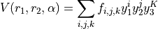
In TROVE, a generic field $f(\xi)$ assumed the following the following compact multi-index representation for a Taylor-type expansion of order $N$ :

(1) $\begin{split} & \lefteqn{f(\xi) \approx \sum_{L=0}^N \sum_{L[{\bf l}]} f_{L[{\bf l}]} (\xi)^{L[{\bf l}]}} \\ & \equiv \sum_{L=0}^N \sum_{l_1=0}^{L}\sum_{l_2=0}^{(L-l_1)} \sum_{l_3=0}^{(L-l_1-l_2)} \sum_{l_{M-1}=0}^{(L-l_1-l_2-\ldots l_{M-2})} f_{ l_1 l_2 l_3 \ldots l_{M} }^{L} \prod_{i} \xi_{i}^{l_{i}} , \end{split}$

where $L[{\bf l}]$ is a set of $\{L,l_1,l_2,l_3,\ldots,l_M\}$ constrained with $l_1+l_2+l_3+\cdots l_M=L$ and $M=3N-6$ . For each set of $\{L, l_1,l_2,\ldots l_{M} \}$ , the index $l_{M}$ given in this equation is redundant and set to

$l_M = L-l_1-l_2-\ldots-l_{M-1}.$

The expansion terms in Eq. (1) are arranged according to their total power $L$ , which defines the perturbation orders $O(\epsilon^L)$ in the expansion of the KEO assuming that each $\xi_\lambda$ is a small displacement from equilibrium of some order of magnitude $\sim O(\epsilon)$ .

We then introduce a mapping of the expansion coefficients $f_{l_1,l_2,ldots,l_M}^L$ for a polynomial of dimension $M$ and expansion order $L_{rm max}$ to a vector $f[i]$ ($i=1,ldots i_{rm max}$)

$f_{l_1,l_2,\ldots,l_M} \to f[n],$

and control the multi-dimension field expansion via a single index $n$

(2) $F(\xi) = \sum_i f[n]\, \xi_1^{i_1} \xi_1^{i_2} \ldots \xi_{i_M}$

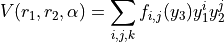
Let us a consider an example of an XY₂ molecule with a PEF given by a typical Taylor-type expansion around a rigid configuration (equilibrium):

$V(r_1,r_2,\alpha) = \sum_{i,j,k} f_{i,j,k} y_1^i y_2^j y_3^K$

where

$\begin{split} y_1 & 1-e^{-a \Delta r_1} \\ y_2 & 1-e^{-a \Delta r_2} \\ y_3 & \Delta \alpha \end{split}$

We now organise this expansion in the form Eq. (1) and present to the second order:

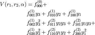
$\begin{split} V(r_1,r_2,\alpha) &= f_{000}^{(0)} + \\ & f_{001}^{(1)} y_3 + f_{010}^{(1)} y_2 + f_{100}^{(1)} y_1 \\ & f_{002}^{(1)} y_3^2 + f_{011}^{(2)} y_2 y_3 + f_{101}^{(2)} y_1 y_3 + \\ & f_{020}^{(1)} y_2^2 + f_{110}^{(2)} y_1 y_2 + f_{200}^{(2)} y_1^2 \end{split}$

Note

The expansion terms are arranged by (1) the total order $L=i+j+k$ and then by the increasing powers of $y_1$ for a given $L$ .

We now map parameter $f_{ijk}^{(L)}$ to a 1D array $f[n]$ with a single index $n=1,n_{\rm max}$ with the total number of polynomial coefficients of

(3) $n_{\rm max} = \frac{(N+1) (N+2) \ldots (N+M)}{M!}$

where $M$ is the number of the internal (expansion) degrees of freedom.

The mapping in our case is organised as follows:

$n$	$i$	$j$	$k$
1	0	0	0
2	0	0	1
3	0	1	0
4	1	0	0
5	0	0	2
6	0	1	1
7	1	0	1
8	0	2	0
9	1	1	0
10	2	0	0

Non-rigid reference configuration

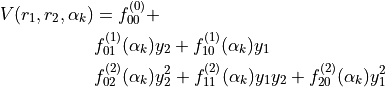
For a non-rigid reference expansion case, a PEF expansion is given by

$V(r_1,r_2,\alpha) = \sum_{i,j,k} f_{i,j}(y_3) y_1^i y_2^j$

around each value of $\alpha$ and $f_{i,j}(y_3)$ are now expansion 1D functions.

Note

Remember that the non-rigid coordinate corresponds always to the last mode, in this case $y_3 = \alpha$ .

The TROVE-form expansion to the second order is now given on a grid of $\alpha_k = [\alpha_{\rm min} \ldots \alpha_{\rm max}]$ :

$\begin{split} V(r_1,r_2,\alpha_k) &= f_{00}^{(0)} + \\ & f_{01}^{(1)}(\alpha_k) y_2 + f_{10}^{(1)}(\alpha_k) y_1 \\ & f_{02}^{(2)}(\alpha_k) y_2^2 + f_{11}^{(2)}(\alpha_k) y_1 y_2 + f_{20}^{(2)}(\alpha_k) y_1^2 \end{split}$

The mapping 3D-to-1D is now as follows

$n$	$i$	$j$	$k$
1	0	0	0
1	0	0	1
1	0	0	2
1	0	0	3
…	…	…	…
2	0	1	0
2	0	1	1
2	0	1	2
2	0	1	3
…	…	…	…
3	1	0	0
3	1	0	1
3	1	0	2
3	1	0	3
…	…	…	…
6	2	0	0
6	2	0	1
6	2	0	2
6	2	0	3

where $k=0\ldots N_{\rm points}$ .

This structure of the mapping is used in TROVE for any arbitrary system of general dimension and also used in the fields’ checkpoints.

potential.chk

The checkpoint file potential.chk containing the expansion parameters $f_{n}(\alpha_k)$ has three sections:

header with a defining the dimensionality.
main body with the expansion values and indexes
footer with a checkpoint “signature”

A potential.chk example for H₂S can be downloaded from potential.chk.

Main body

For the example of a 2nd order expansion, the body of potential.chk has the following structure:

      0  0.1204141314001783E-03
      0  0.2530099244534204E+01
      0  0.7599034116321027E+01
      0  0.7599034116321026E+01
      0  0.1909437919650396E+05
      0 -0.2632308040173431E+04
      0  0.3714665204913049E+05
      0 -0.2632308040173436E+04
      0 -0.3464213699036532E+03
      0  0.3714665204913049E+05

Where

col 1: the 1D expansion index $n$ ;
col 2: the non-rigid expansion index :max:`k = 0\ldots N_{\rm points}` ( $N_{\rm points} = 0$ for the Rigid case);
col 3: the value of the expansion parameter $f_{n}(\alpha_k)$ .

Note

The format is not sensitive to the exact position of the columns the exact format of the values in the last column with spaces as separators between then. The order of the column however is important, but the order of the rows is not!

Footer

The footer of potential.chk (and of other fields) is used to (i) indicate the end of the main body part and (ii) for a general control of the correctness of the file structure. It also reports the value of the coefficient threshold $f_{\rm min}$ used to prune the potential expansion from parameters wit very small values. It has the following generic format:

  987654321     0 0.00000000000E+00 <- End
 0.10000000E-23      <- sparse threshold used
End of potential

Here:

987654321 is a signature card indicate the end of the main body section. The values in columns 2 and 3 are dummy and only used to maintain the structure when reading potential.chk line-by-line.
0.10000000E-23 is the coefficient threshold value $f_{\rm min}$
End of potential is an obligatory (case sensitive) signature at the end of the file. It is used to check the correctness of the input.

The input fields <- End and <- sparse threshold used are ignored by the TROVE read and only for clarity.

For a non-rigid XY₂ case with $N_{\rm order}=2$ , the structure of potential.chk is as follows (for $N_{\rm points}^{\rm max} = 3$ ):

     0      2.1950703863E+06
     1      2.1950667601E+06
     2      2.1950558811E+06
     3      2.1950377475E+06
     0      1.0824765910E+03
     1      1.0822716655E+03
     2      1.0816568852E+03
     3      1.0806322393E+03
     0      1.0824765910E+03
     1      1.0822716655E+03
     2      1.0816568852E+03
     3      1.0806322393E+03
     0     -3.9896888537E+06
     1     -3.9896813769E+06
     2     -3.9896589454E+06
     3     -3.9896215557E+06
     0      6.2738693377E+04
     1      6.2739094227E+04
     2      6.2740296812E+04
     3      6.2742301244E+04
     0     -3.9896888537E+06
     1     -3.9896813769E+06
     2     -3.9896589454E+06
     3     -3.9896215557E+06

Kinetic Energy Operator checkpoint

The KEO has the following general form:

(4) $\begin{split} \hat{T} &= \frac{1}{2} \, \sum_{\alpha=x,y,z} \; \; \sum_{\alpha^\prime=x,y,z} \hat{J}_{\alpha}\, G_{\alpha,\alpha^\prime}^{\rm rot}(\xi)\, \hat{J}_{\alpha^\prime} \\ &+ \, \sum_{\alpha=x,y,z}\;\; \sum_{n=1}^{3N-6} \left[ \hat{J}_{\alpha}\, G_{\alpha,\lambda}^{\rm Cor}(\xi)\, \hat{p}_\lambda + \hat{p}_\lambda \, G_{\alpha,\lambda}^{\rm Cor}(\xi)\, \hat{J}_{\alpha} \right] \\ &+ \, \sum_{\lambda=1}^{M}\; \sum_{\lambda^\prime=1}^{M} \hat{p}_\lambda \, G_{\lambda,\lambda'}^{\rm vib}(\xi)\, \hat{p}_{\lambda'} + U(\xi), \end{split}$

It consists of four main components, rotational, Coriolis, vibrational and Pseudo-potential, represented by the corresponding KEO expansion terms $G_{\alpha,\alpha^\prime}^{\rm rot}$ , $G_{\alpha,\lambda}^{\rm Cor}$ , $G_{\lambda,\lambda'}^{\rm vib}$ and $U$ . Each of them is then represented by a Taylor-type expansion of Eq. (1), either around a rigid configuration ( $N_{\rm points}=0$ ) or a non-rigid one.

The multi-dimension expansions are mapped to a 1D array using the same structure as described for PEFs. The corresponding KEO parameters are saved in the checkpoint file kinetic.chk using the same format with additional specifiers for the KEO term indexes, e.g. $\lambda,\lambda'$ as in $G_{\lambda,\lambda'}^{\rm vib}$ as well as to indicate which expansion component they belong to.

The kinetic.chk file is organised into four parts, vibrational, rotational, Coriolis and pseudo-potential (in this order). A kinetic.chk example for H₂S can be downloaded from kinetic.chk.

As an example to illustrate its structure , let us use the example of XY₂ again assuming the expansion order of $N=0$ (rigid rotor KE). Each par ends with a one footer line:

987654321     0        0        0  0.00000000E+00 <- End

as described for potential.chk, and after the last section, the file ends with the footer:

 0.10000000E-23      <- sparse threshold used
End of kinetic

Note

Here End of kinetic is a case sensitive obligatory string on the very last line, treated as three words End, of and kinetic with spaces as decimeters.

The first part of kinetic.chk has the following format

      2       1           <- g_vib Npoints,Norder,Ncoeff
  ----- ------  ------- ------- -----------------------
  col 1  col 2   col 3   col 4          col 5
  ----- ------  ------- ------- -----------------------
   1       1       0        3.45080007E+01
   2       1       0       -4.16924395E-02
   3       1       0        7.88754390E-01
   1       1       0       -4.16924395E-02
   2       1       0        3.45080007E+01
   3       1       0        7.88754390E-01
   1       1       0        7.88754390E-01
   2       1       0        7.88754390E-01
   3       1       0        3.87191518E+01
   1       1       0        2.07473906E+01
   2       1       0        9.64742256E+00
   3       1       0        1.80323802E+01
   0       1       0       -6.05339917E+00
    ...............
987654321     0        0        0  0.00000000000E+00 <- End

col 1: the value of the index $\lambda$ in $G_{\lambda,\lambda'}^{\rm vib}$
col 2: the value of the index $\lambda'$ in $G_{\lambda,\lambda'}^{\rm vib}$
col 3: expansion index $n$ in Eq. (2).
col 4: The non-rigid grid point $k$ ( $\alpha_k$ ), zero for the rigid and $k=0\ldots N_{\rm ponits}$
col 5: Value of the expansion parameter $g_{\lambda,\lambda'}[n](\alpha_k)$ .

The vibrational part is followed by the rotational part using the same structure:

    0        2        0          <- g_rot Npoints,Norder,Ncoeff
  ----- ------  ------- ------- -----------------------
  col 1  col 2   col 3   col 4          col 5
  ----- ------  ------- ------- -----------------------
     1     1       1       0        2.07473906E+01
     2     2       1       0        9.64742256E+00
     3     3       1       0        1.80323802E+01
    ...............
987654321     0        0        0  0.00000000000E+00 <- End

col 1: the value of the index $\alpha$ in $G_{\alpha,\alpha'}^{\rm rot}$
col 2: the value of the index $\alpha'$ in $G_{\alpha,\alpha'}^{\rm rot}$
col 3: expansion index $n$ in Eq. (2).
col 4: The non-rigid grid point $k$ ( $\alpha_k$ ), zero for the rigid and $k=0\ldots N_{\rm ponits}$
col 5: Value of the expansion parameter $g_{\alpha,\alpha'}[n](\alpha_k)$ .

For the zero-order expansion, only the diagonal elements are present in the KEO of XY₂.

The next part of kinetic.chk list the expansion parameters of $G_{\alpha,\lambda}^{\rm Cor}$ . Sice this part is absent for the zero order expansion case, let us increase $N$ to 1 for the sake of an illustration:

    0        1       4           <- g_cor Npoints,Norder,Ncoeff
  ----- ------  ------- ------- -----------------------
  col 1  col 2   col 3   col 4          col 5
  ----- ------  ------- ------- -----------------------
     1    2        2       0       -6.44399927E+00
     1    2        3       0       -1.47113686E-01
     1    2        4       0        1.47113686E-01
     2    2        2       0        6.44399927E+00
     2    2        3       0       -1.47113686E-01
     2    2        4       0        1.47113686E-01
     3    2        3       0       -7.22166143E+00
     3    2        4       0        7.22166143E+00
    ...............
987654321     0        0        0  0.00000000000E+00 <- End

col 1: the value of the index $\alpha$ in $G_{\alpha,\lambda}^{\rm Cor}$
col 2: the value of the index $\lambda$ in $G_{\alpha,\lambda}^{\rm Cor}`$
col 3: expansion index $n$ in Eq. (2).
col 4: The non-rigid grid point $k$ ( $\alpha_k$ ), zero for the rigid and $k=0\ldots N_{\rm ponits}$
col 5: Value of the expansion parameter $g_{\alpha,\lambda}[n](\alpha_k)$ .

The last, pseudo-potential part, contains expansion coefficient of $U(\xi)$ . For the $N=1$ case it is given by:

      1       4          <- pseudo Npoints,Norder,Ncoeff
   0        1        0  -0.605339916936254152E+01
   0        2        0   0.494666955682775800E+00
   0        3        0   0.453132419899363814E+01
   0        4        0   0.453132419899363725E+01
987654321     0        0        0  0.00000000000E+00 <- End

cols 1-2: two dummy zero values just to keep the same structure as above
col 3: expansion index $n$ in Eq. (2).
col 4: The non-rigid grid point $k$ ( $\alpha_k$ ), zero for the rigid and $k=0\ldots N_{\rm ponits}$
col 5: Value of the expansion parameter $u[n](\alpha_k)$ .

The final part is the footer as examined above:

 0.10000000E-23      <- sparse threshold used
End of kinetic

Extended format of kinetic.chk

In the case of the Basic-Function feature used, the kinetic.chk format is required to contain the individual exponents for all modes of each term explicitly. For details, see Kinetic energy operators. The extended format has now the following form (example for the g_vib section):

 7   93    <--- Gvib Npoints,Norder,Ncoeff
   1     1   0   3.86412653967     0    0    0    0    0    0
   2     1   0   2.80960448197     0    0    0    1    0    0
   3     1   0   2.80960448197     0    0    0    0    1    0
   4     1   0  -2.80960448197     0    1    0    4    0    0
   5     1   0  -2.80960448197     0    0    1    0    4    0
   6     1   0               0     0    0    0    0    0    0
   1     1   0   2.80960448197     0    0    0    1    0    0
   2     1   0   36.2630831225     0    0    0    0    0    0
.....

where the first three integer numbers Npoints,Norder,Ncoeff are as before, $N_{\rm points}$ , $N_{\rm order}$ and $N_{\rm coeff}$ , respectively with one important difference. $N_{\rm coeff}$ is the number of non-zero coefficients. The columns of the main body are as follows:

----- ----- ---- --- ---------------- ---- ---- ---- ---- ----- ----
  1     2     3   4           5         6    7    8    9    10   11
----- ----- ---- --- ---------------- ---- ---- ---- ---- ----- ----
  1     1     1   0   3.86412653967     0    0    0    0    0    0
  1     2     1   0   2.80960448197     0    0    0    1    0    0
  1     3     1   0   2.80960448197     0    0    0    0    1    0
  .....

The first 5 columns are as before:

col 1: the value of the index $\lambda$ in $G_{\lambda,\lambda'}^{\rm vib}$
col 2: the value of the index $\lambda'$ in $G_{\lambda,\lambda'}^{\rm vib}$
col 3: expansion index $n$ in Eq. (2).
col 4: The non-rigid grid point $k$ ( $\alpha_k$ ), zero for the rigid and $k=0\ldots N_{\rm ponits}$
col 5: Value of the expansion parameter $g_{\lambda,\lambda'}[n](\alpha_k)$ .

The rest 6 columns contain the corresponding exponents of each mode in Eq. (2).

col 6: $i_1$
col 7: $i_2$
col 8: $i_3$
col 9: $i_4$
col 10: $i_5$
col 11: $i_6$ (i.e. $i_M$ ).

External field checkpoint

This is a genial purpose field, used for example to store the dipole moment, correction to the PEF in the refinement etc. It is assumed to be a 1D array of the dimensionality $D$ ( $D=3$ for the dipole).

It follows the same structure as above, just with one index representing the field component. For example:

      6       28        3          <- Npoints,Norder,Ncoeff,Rank
      1        0 -0.7458479825692242E+00
      1        1 -0.7491358566222752E+00
      1        2 -0.7524174492956430E+00
      1        3 -0.7556927371155667E+00
      1        4 -0.7589616967156357E+00
      1        5 -0.7622243048371204E+00
      1        6 -0.7654805383293001E+00
............

In the first line here, the last number specifies the dimensionality of the field (here 3).

As before, the checkpoint file ends with the footer

  987654321     0        0  0.00000000000E+00 <- End
 0.00000000E+00      <- no sparse was threshold used
End of external

An external.chk example for H₂S can be downloaded from external.chk.

Checkpoints

List of checkpoints

“Fingerprints”

Structure of the description checkpoints

contr_descr.chk

eigen_descr*_*.chk

j0eigen_descr*_*.chk

Potential, Kinetic and External (dipole) checkpoints

Non-rigid reference configuration

potential.chk

Header

Main body

Footer

Kinetic Energy Operator checkpoint

Extended format of kinetic.chk

External field checkpoint

`contr_descr.chk`

`eigen_descr_.chk`

`j0eigen_descr_.chk`