Line lists and Spectra

This chapter will give details on how to use TROVE and associated programs to make production quality line lists and spectra. That is, large line lists involving millions or even billions of transitions between states. The programs involved are called GAIN and Exocross. Both have been designed to interface with TROVE outputs and using them does not require much additional syntax.

Intensity calculations are a part of step 4 (see Chapter Quickstart for the description of TROVE steps an Chapter Theory for theoretical details of the intensity calculations).

Prerequisites of intensity calculations in TROVE

We assume that all three initial steps have been accomplished. This includes: solution of the ro-vibrational problem by computing the ro-vibrational wavefunctions $\Psi_{\rm rv}^{(i)}$ and energy term values $\tilde{E}_i$ , steps 1-3. The wavefunction coefficients $C_{v'' k'' }^{(i)}$ are stored in the check points j0eigen_vectors*.chk, while the energies are in the ascii files j0eigen_descr*.chk for a set of $J$ from 0 to $J_{\rm max}$ . We also assume that the DMS components have fully been processed in steps 1 and 2. At step 1 this incudes (i) definition of DMS in the step 1 input file, (ii) re-expansion in terms of the TROVE internal vibrational coordinates (external.chk) and (iii) calculation of the vibrational matrix elements of the DMS components (extmatelem1.chk, extmatelem2.chk and extmatelem3.chk). At step, the DM matrix elements are converted to the $J=0$ representation (j0_extmatelem1.chk, j0_extmatelem2.chk and j0_extmatelem3.chk). Providing that these ingredients are available, the intensities can be generated as follows.

INTENSITY input file: step 4

In order to start the intensity calculations, the following changes in the input are required. In the CONTROL section, the keyword step has to be set to 4 and the range of the values of $J$ needs to be defined, e.g.

Control
Step 4
J 0 10
end

Besides, an INTENSITY section has to be added anywhere in the input (see Quickstart), e.g.

 INTENSITY
  absorption
  exomol
  linelist *filename*
  THRESH_INTES  1e-20
  THRESH_LINE   1e-20
  THRESH_COEFF  1e-18
  TEMPERATURE   300.0
  Partition     1000.0
  GNS          8.0 8.0 8.0
  selection (rules) 1 1 2  (N of irreps)
  freq-window  -0.1,   4000.0
  energy low   -0.1,  2000.0, upper   -0.1, 6000.0
END

Here absorption specifies that absorption intensities between states are to be calculated.

THRESH_INTES/LINE/COEFF are used to control the level of print out for intensities. Very large outputs can be produced if these are set very low (as needed for ‘production’ quality line lists) but for quicker checks higher values should be used. The intensities are evaluated and checked for the reference temperature value specified.

TEMPERATURE is used to specify the reference temperature used to evaluate the intensities and also check them against the threshold value THRESH_INTES. It should be noted that the main product of the ‘Intensity’ calculations are the temperature independent Einstein coefficients and therefore temperature does play any role. It is only used for (i) a quick intensity check when the intensities are printed out in the standard output file (not exomol format) and a reference temperature is needed or (ii) to apply the intensity threshold. For the latter it can be seen as the maximal temperature in conjunction with the lower state energy threshold and $J_{\rm max}$ . Once the Einstein coefficients are produced, any temperature can be in principle used to simulate intensities using e.g. ExoCross.

Partition is the reference value of the partition function $Q(T)$ . It is used to evaluate the intensities in connection with the reference temperature as explained above. Although in principle, TROVE’s calculated values could be used to evaluate the value of $Q(T)$ , in practice the intensity calculations are split into sub-ranges of $J$ and therefore the full set of energies is not always known for accurate evaluation of $Q(T)$ . As reference values needed for the intensity threshold purposes, even a very rough estimate is sufficient. For the transition moments TM, this corresponds to the vibrational $Q(T)$ .

GNS is the state dependent spin statistical weights $g_{\rm ns}^{(i)}$ for each symmetry (irrep). These can be looked up for many molecules or worked out from the procedure in Bunker and Jensen, chapter 8 [98BuJe]. The $g_{\rm ns}$ value is used directly in the intensity calculations if required as well as to evaluate the total degeneracy for States file outputs, $g_{\rm tot}^{(i)} = J(J+1) g_{\rm ns}^{(i)}$ .

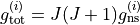selection-rules is used to specify selection rules, i.e. which symmetries can make up the initial and final states of a transition. The product of the upper and lower eigenfunctions must contain a component of the dipole itself [98BuJe]. Let’s consider a symmetry group spanning $N_{irrep}$ irreps $\Gamma_1. \Gamma_2, \ldots$ (which we denote in TROVE with integers 1,2,3,4…) with the selection rules

$\Gamma \leftrightarrow \Gamma'$

Here $\Gamma'$ is the allowed irrep partner for $\Gamma$ .

selection-groups (selection) is an alternative way to specify the selection rules by defining groups of allowed transitions they belong to. Thus for the PH₃ example, $A_1$ and $A_2$ are grouped together while $E$ can only go to $E$ . Integers are used to form groups, in this case 1 1 are for $A_1$ and $A_2$ and 2 is for E. The selection card is then given by

1 1 2

for $A_1$ , $A_2$ and $E$ , respectively.

The selection-rule ‘card’ has then the following format

$i_{\Gamma'_1} i_{\Gamma'_2} i_{\Gamma'_3} i_{\Gamma'_4} \ldots$

where $i_{\Gamma'_1}$ is the ID of the allowed irrep partner for the irrep 1, $i_{\Gamma'_2}$ is the ID of the allowed irrep partner for the irrep 2 etc. For example, for a C_3v molecule like PH₃, spanning $A_1$ (irrep 1), $A_2$ (irrep 2) and E (irrep 3) with the selection rules

$\begin{split} A_1 &\leftrightarrow A_2 \\ A_2 &\leftrightarrow A_1 \\ E & \leftrightarrow E \\ \end{split}$

it is given by

2 1 3

J, i,j specifies the rotational states to be included. In the example above 0 to 10 were used. It is often better to split a calculation into 0,1-1,2-2,3, etc to fit into time allocations on computers. The vibrational states to be included can also be specified by the v i, lower x, y, upper x', y' where i is the number of a vibrational mode and x, x’ and y, y’ give the limits for the lower and upper states included. If this is not included then all vibrational states are considered.

freq-window This specifies the frequency window (in wavenumbers) in the spectra to be used. In the example here -0.1 is used as the minimum to guarantee values from 0 are used while 4000 is the maximum considered. energy low specifies the energies of the lower and upper states to be included. In the example the highest energy lower state to include it 2000 so since the maximum frequency of light considered is 4000, the upper state needs a maximum of 6000 (energy proportional to frequency, $E = h \nu$ ).

exomol is the keyword to produce a line list in the ExoMol format, which will be written into the .trans and .states files. In this case, the absorption intensities computed for the temperature and partition functions specifies are not printed out only used together with the corresponding threshold THRESH_INTES to decide to keep the line in the line list or not.

linelist is the filename of the .trans and .states files.

To calculate absorption intensities the eigenfunctions and eigenvalue files of the states to be included must be included in the directory where TROVE is run. More on this will be described below.

states_only card is used to produce the States file only. It can be used to collect all the states into a single file.

symmetry reduced card in the Intensity section is to switch on the reduced treatment of the degenerate symmetry components of the ro-vibrational wavefunctions when calculating the line strength and thus safe time. In particular, the ro-vibrational matrix elements of the dipole moments between degenerate symmetry components $\Gamma_\alpha$ have the following properties

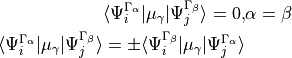
$\begin{split} \langle \Psi_{i}^{\Gamma_\alpha} |\mu_{\gamma}| \Psi_{j}^{\Gamma_\beta} \rangle = 0, & \alpha = \beta \\ \langle \Psi_{i}^{\Gamma_\alpha} |\mu_{\gamma}| \Psi_{j}^{\Gamma_\beta} \rangle = \pm \langle \Psi_{i}^{\Gamma_\beta} |\mu_{\gamma}| \Psi_{j}^{\Gamma_\alpha} \rangle \end{split}$

therefore only one non-diagonal component is unique and needs to be computed.

Note

When invoking this option, it is advised to check that the results are the same.

Choosing threshold values

The intensity block in TROVE requires a choice for the minimum intensities to be printed out and for the range of states and frequencies to be included. The value of intensity thresholds should be set very small for production quality line lists, for example THRESH_INTES and THRESH_LINE can be set at $1\times 10^{-50}$ to ensure all transitions are included.

Values for freq-window and energy low and upper depend on the molecule and temperature of interest. The lower energy range required will depend on the desired temperature range. For room temperature line lists, only relatively low energy states will be significantly populated. For hot line lists, this range will be increased. The partition function for the molecule can be used to judge which states are required for coverage at a certain temperature (see below for how to calculate using ExoCross). The frequency window (and thus upper states to include) depends on the frequency of light which of interest. Of course, the range which is included will also be limited by practical considerations such as computational time, memory, basis set convergence, etc.

Restarting unfinished intensity jobs

The line intensity calculations are organised as follows. First, energies selected for a given run are combined, sorted and renumbered. Here is an example of such as selection:

J, 20,      21
freq-window  0,12000
energy low   0,10000.0, upper  -0.00,18000.0

Then, the intensities are processed in batches divided by lower states: each batch corresponds to transitions from a given lower state to all upper states in a given selection. Within each batch, the calculations are OpenMP parallelised. In large projects, it is common that a given selection does not fit into the wall-clock limit of an HPC the job selection needs to be divided into sub-selection. The most natural way is to divide jobs by the lower states by energy ranges, e.g. 0 to 1000 1/cm, 1000.0001 to 2000, 2000.0001 to 3000 etc. However such selection is uneven. The higher the range the more transitions it corresponds to.

A more efficient way to divide a selection into sub-selections is by the lower state count. Before introducing this concept, let first define the following useful card.

wallclock gives control of the calculation time and prevents crashing when running on an HPC scheduler with a time limit (wallclock time):

   wallclock 32.0

By setting ``wallclock`` to a value in hours which is less than the HPC wallclock, TROVE will do a control stop and report marks describing the calculation stage to be used in the restart. When time is close to wallclock, TROVE will let the current group (all transitions starting from the same lower state) of intensities to finish and provide the following report (e.g.):

... [wall-clock stop]: last lower-state     1189 out of            15462 (           15462), processed =     1189 states;
... last energy =     10140.830465

...Intensities finished: From        1 to     1189 of    15462 lower states.

Here,

1 is the counting number of the 1st lower state selected for the current run;

1189 is the counting number of last lower state finished;

15462 is the total number of the lower states selected for the current run (and available);

1189 is the number of states prossed during the current run;

10140.830465 is the value (1/cm) of the last lower state processed.

One can assume that each line takes approximately the same time, for a given set of $J'$ and $J''$ . These numbers also tell how many lower states can fit into one wallclock limit and thus can help divide the intensity jobs into sub-groups, organised by the lower states. Here, e.g., it is 1189 states per one wallclock limit. We can therefore divide the intensity jobs e.g. by 1049 (smaller than 1189 just in case):

1190-2239
2240-3289
3290-4339
4340-5389
5390-6439
6440-7489
7490-8539
8540-9589
9590-10639
10640-11689
11690-12739
12740-13789
13790-14839
14840-15462

For the restart the first batch, the following card needs to be used:

count  1190 2239

If the jobs has fully completed, the following printout will appear at the end of the standard TROVE output file:

...Intensities finished: From     1190 to     2239 of    15462 lower states.

Otherwise, the print out information can be used to restart this batch again.

Line list format

States file

A typical States file has the following format:

-----  ----------- ------- ------ ----  --- -- --- --   --- -- --  ------ --    ------- -- -- --  -------
    1       2           3       4   5     6  7  8  9    10  11 12     13  14        15  16 17 18       19
-----  ----------- ------- ------ ----  --- -- --- --   --- -- --  ------ --    ------- -- -- --  -------
    1     0.000000      1       0  A1     0  0  0  A1    0   0 A1    1.00 ::         1   0  0  0        1
    2  1172.667646      1       0  A1     0  0  1  A1    0   0 A1    1.00 ::         2   0  0  1        2
    3  2335.297519      1       0  A1     0  0  2  A1    0   0 A1    1.00 ::         3   0  0  2        3
    4  2608.713940      1       0  A1     1  0  0  A1    0   0 A1    1.00 ::         4   1  0  0        4
    5  3503.042415      1       0  A1     0  0  3  A1    0   0 A1    1.00 ::         5   0  0  3        6
    6  3765.459944      1       0  A1     1  0  1  A1    0   0 A1    1.00 ::         6   1  0  1        7
    7  4675.006191      1       0  A1     0  0  4  A1    0   0 A1    1.00 ::         7   0  0  4        9
    8  4927.853585      1       0  A1     1  0  2  A1    0   0 A1    1.00 ::         8   1  0  2       10
    .......
    .......

where the designation of the columns is as follows

Col 1: is the State ID (integer);

Col 2: Energy term value of the state;

Col 3: g_tot is the total degeneracy of the ro-vibrational state;

Col 4: J is the total angular momentum rotational quantum number;

Col 5: G_tot is the total symmetry of a ro-vibrational state;

Cols 6-8: v1, v2, v3 are the TROVE (local mode) vibrational quantum numbers;

Col 9: Gv is the vibrational symmetry of the vibrational contribution;

Col 10: k is a rotational quantum number (projection of $J$ on the molecular axis $z$ );

Col 11: t is a rotational index defining the state parity $\tau$ ;

Col 12: G_r is the rotational symmetry;

Col 13: C_i is the largest eigen-coefficient used in the assignment.

Col 14: :: label to indicate States, not repeated in other States file, can be used to grep unique entries;

:; label to indicate States, that repeat in other States file. Only unique for the J=Jmax last calculation and can be used to grep and add to the fill set of State entries;

Col 15: J-Symmetry-Block counting number

Cols 16-18: Normal mode quantum number n1, n2, n3 if introduced in contr_descr.chk at step 2. Otherwise can be ingored.

Col 19: Vibrational counting number as appear in the j0contr_descr.chk file.

The separator labels :: and :; are introduced to avoid double counting when combining States file from intensity calculations covering different ranges of $J$ . As discussed above, a given calculation for $J = [J_1,J_2]$ does not include transitions between $J''=J_1$ and $J' = J_1$ (lower bound), but includes transitions between $J''=J_2$ and $J' = J_2$ (upper bound). the next interval to be considered is for $J = [J_2,J_3]$ , which thus also produces a States file with the same states $J=J_2$ . When combining states multiple file, in order to avoid double counting, one can grep all state with the label :: first

grep -h "::" *.states > All.states

and then add states from the very last $J = J_{\rm max}$ by grepping :;:

grep ":;"  Last_Jmax.states >> All.states

Alternatively, one can simply run an intensity calculation with the states-only keyword for the entire range at once (here for $J_{\rm max}=100$ ):

Control
Step 4
J 0 100
end

Besides, an INTENSITY section has to be added anywhere in the input (see Quickstart), e.g.

 INTENSITY
  absorption
  states-only
  exomol
  linelist filename
  .....
  freq-window  -0.1,   -1.
  energy low   -0.1,  2000.0, upper   -0.1, 6000.0
END

Transition file

A typical transition file has the following format:

------- ------------ ---------------    --------------
   1             2           3                 4
------- ------------ ---------------    --------------
   49            1    5.03640979E-04        17.228535
   50            1    1.42153137E-02      1190.140067
   51            1    1.56245751E-02      2353.041332
   52            1    2.24850939E-02      2626.439267
   53            1    1.70424762E+00      3318.238716
------- ------------ ---------------    --------------

where

col 1: the upper state ID as in the States file(s);

col 2: the lower state ID;

col 3: Einstein A coefficient (1/s);

col 4: Transition wavenumber(cm^-1).

Different functionality of INTENSITY

The card PRUNING is for building an intensity (transition-moment, TM) list used for intensity (TM) pruning (see Additional Features about the basis set pruning).

TDM_REPLACE (DIPOLE_REPLACE, DIPOLE_SCALE) is for scaling the vibrational transition dipole moments for individual bands in order to improve the agreement with experimental intensities. The scaling factors must be stored in the file j0_tdm.chk in the following format:

i1 i2 factor

where i1 and i2 are the vibrational state indexes as in j0contr_descr.chk for a given band and factor is the factor to scale.

ZPE: a ZPE can be specified directly in the INTENSITY block.

Intensities with GAIN

As discussed in Chapter Quickstart, TROVE is capable of calculating transition intensities once the relevant eigenfunctions and dipole matrix elements have been calculated. This procedure was used in early line list papers using TROVE.

A more efficient way of calculating intensities is to make use of the GAIN program. GAIN (GPU Accelerated INtensities) is a program which was written by Ahmed Al-Rafaie (see GAIN_). It uses graphical processing units (GPUs) to calculate intensities far quicker than can be achieved using conventional TROVE.

GAIN uses the same input file as TROVE but only the intensity block is actually used to control the calculation. GAIN requires the eigenvectors, eigen description and eigen quanta files for the states of interest. It also requires the eigen descrption and eigen quanta of the $J = 0$ state and extfield file for the dipole matrix elements (note that currently GAIN cannot accept split dipole files, these must be stitched together).

GAIN can be found at gitGAIN.

Using GAIN

The number of states for a polynomial molecule quickly increases with $J$ and energy. This leads to millions of transitions and so even with GAIN, intensity calculations scale quite drastically. There are a few ways in which calculations can be sped up however so that they can be run within wall clock limits.

The first is to increase the number of nodes used. GAIN is an mpi parallel program and can make use of multiple nodes, which themselves have multiple cores. A rule of thumb for how many cores to use is: size of eigenvectors / memory available per core.

Another speed increase is to split the intensities which are being calculated by $J$ and symmetry. Rotational selection rules limit transitions to $J'' = J'$ and $J'' = J' \pm 1$ . Currently GAIN does not have a rule for only computing upper or lower Q branch transitions and so these duplicates should be removed for a complete line list. Using the selection rule, intensities can be calculated by setting $J$ in the intensity block to 0,1 then 1,2 then 2,3, etc. Symmetry also limits transitions but these are molecule dependent. For example, for PF₃ transitions can only take place for $A_1$ $\leftrightarrow$ $A_2$ and E $\leftrightarrow$ E. To make use of this symmetry the nuclear statistical weights ( $g_{ns}$ ) for the symmetries which are allowed should be set to their usual values but others set to 0. For example for $A_1 \leftrightarrow A_2$ in PF₃ the $g_{\rm ns}$ would be set to 8.0 8.0 0.0. For both $J$ and symmetry selection rules, a separate input file and run of GAIN should be carried out for each selection rule.

GAIN produces two types of output files. The .out files begins with a repeat of the input file. Information is then given on which .chk files were opened and which GPUs are being used and their memory. Information is then given on how GAIN splits up the calculation and how many transitions are to be computed. GAIN then cycles through the energy states starting with the lowest energy and computes all transitions to higher energies. For each complete lower energy calculation the current lines per second computed (L/s) is reported along with the predicted total time required. The other output file produced is a __n__.out file. Here n is an integer starting at 0 going up to number of nodes $-1$ . This file(s) contain the GAIN results and lists the frequency and the Einstein A coefficient cite{98BuJexx} for a transition. Labels are also given for which states the transition is between.

Einstein A coefficients are calculated as opposed to intensities as these are temperature (and pressure) independent. To simulate and plot a spectrum Exocross is used which is discussed in the next section.

Currently the format for the intensities from GAIN is not compatible with Exocross. Programs can be used however to convert the GAIN output to the slightly more compact Exomol format. Code for doing this can be obtained from Sergey Yurchenko. In the future it may be that GAIN is modified to directly output the correct format for Exocross.

The intensity format of MPI GAIN is as in the following example:

------------  ------  ----  ---       ----- ---  ---  ---------------  --
        2      3    4           5    6    7          8        9
------------  ------  ----  ---       ----- ---  ---  ---------------  --
655690     6568   36    5 <-        1   36    4  1.463207104E-08  ||
676249    12215   36    5 <-        1   36    4  1.182320455E-05  ||
982789    13452   37    5 <-        1   36    4  1.462048511E-09  ||
662096    42951   37    5 <-        1   36    4  1.439647858E-05  ||
929053    12600   37    5 <-        1   36    4  3.588055083E-09  ||
333158    40203   37    5 <-        1   36    4  2.714626451E-06  ||
326880    15974   36    5 <-        1   36    4  2.652568503E-07  ||
493882     7351   37    5 <-        1   36    4  2.458227845E-08  ||
559823     2479   37    5 <-        1   36    4  5.619855017E-08  ||
227725      826   37    5 <-        1   36    4  7.447377296E-09  ||
981779    12218   36    5 <-        1   36    4  2.205478079E-07  ||
....

where

col 1: Transition wavenumber(cm^-1);
col 2: upper state counting ( $J-\Gamma$ -block) number;
col 3: upper state $J$ .
col 3: upper state symmetry $\Gamma$ .
col 5: lower state counting ( $J-\Gamma$ -block) number;
col 6: lower state $J$ .
col 7: lower state symmetry $\Gamma$ .
col 8: Einstein A coefficient (1/s);
col 9: “||” label to help extracting and combining intensity entries from the GAIN outputs.

The same format can be used in TROVE, which is invoked by the keyword GAIN in the step 4 INTENSITY as in the following card:

GAIN

Exocross

As discussed above, GAIN produces a list of temperature and pressure independent Einstein A coefficients. To simulate a spectra, these must be converted into intensities. This can be achieved using ExoCross [ExoCross], providing the data is correctly formatted. TROVE can directly produced intensities but ExoCross has features which make it a better choice for production quality simulations.

To run ExoCross, two types of file are required. A TRANS file which contains information about the intensity of transitions and a STATES file which contains the energy levels of the molecule. These files should be obtained using a program to change GAIN output or from TROVE directly. This is likely to change depending on situation and will not be discussed here.

A simple but important calculation which can be performed using ExoCross is finding the partition function at a given temperature. This is determined from the States file only. An example input is

mem 63 gb

partfunc
 ntemps 10
 tempmax 800 (K)
end

NPROCS 12

verbose 4

States C2H4_v01.states

The keyword partfunc is used to select a partition function calculation. ntemps is the number of partitions of the temperature, tempmax which will be calculated. For this example the partition function will be calculated at 80, 160, … and 800 K. verbose is the level of print out. States is the name of the states file.

The output for this calculation is simple. A repeat of the input is first given and then the partition function calculation for each temperature is given in columns. The running total of the partition function with $J$ is given in rows.

ExoCross can also be used to make a stick spectrum`. This is an idealised spectrum where each absorption is only represented by a line at a given wavenumber and intensity and broadening effects (doppler, collision, etc) are ignored. An input example is

mem 63.0 gb

Temperature  296
Range 0 9000.0

Npoints 90001

absorption
stick

mass 28
threshold 1e-25

pf 11000.0


output C2H4_thr_1e-25_T296

ncache 1000000

NPROCS 16

verbose 4

States C2H4_v01.states

Transitions
 c2h4_initial_vib_2016_intense_j0_j1__0__.out_0.-9000..trans
 c2h4_initial_vib_2016_intense_j1_j2__0__.out_0.-9000..trans
 ...
 ...
end

Temperature is the temperature of interest in Kelvin.

Range specifies the wavelength range to be used, in this case 0 to 9000 cm^-1.

Npoints controls the density of the grid produced. In this example there will be 10 points per cm^-1.

absorption specifies that a spectra is to be computed and stick indicates that a stick spectrum is required.

mass is the molecule’s mass in atomic mass units.

threshold is the minimum intensity of transition to be included. This is important for keeping the output file manageable so it can be used for making plots.

pf is an optional keyword which is used to give the value of the partition function rather than calculate it from the States file (the default case). This is useful if, for example, not all $J$ have been calculated but you want to check the spectrum looks reasonable.

output specifies what to call the output file.

ncache is how much memory will be cached on the cpu during calculations. nprocs is the number of threads to use.

States is the States file to use and Transitions is a list of Trans files to use.

ExoCross has other options for simulating spectra. Examples include accounting for line broadening by using Gaussian or Voigt profiles for each line. The effects of particular background gas collisions can also be taken into account. These features are fully discussed in a recent publication and manual for the ExoCross program and the reader is directed there for full details [ExoCross].