Potential energy functions
TROVE provides a larger number of potential energy functions (PEFs) for different molecules already implemented. Most of these PEFs are in modules pot_* contained in file pot_*.f90.
pot_xy2.f90
pot_xy3.f90
pot_zxy2.f90
pot_abcd.f90
pot_xy4.f90
pot_zxy3.f90
These are a part of the standard TROVE compilation set. Alternatively, a user-defined PEF can be included into the TROVE compilation as a generic ‘user-defined’ module pot_user, see details below.
Potential Block
The Potential (Poten) block used to specify a PEF, has the following generic structure (using XY2 as an example)
POTEN
NPARAM  102
POT_TYPE  POTEN_XY2_MORSE_COS
COEFF  list  (powers or list)
 RE13         1  0.15144017558000E+01
 ALPHAE       1  0.92005073880000E+02
 AA           1  0.12705074620000E+01
 B1           1  0.50000000000000E+06
 B2           1  0.50000000000000E+05
 G1           1  0.15000000000000E+02
 G2           1  0.10000000000000E+02
 V0           0  0.00000000000000E+00
 F_0_0_1      1 -0.11243403302598E+02
 F_1_0_0      1 -0.94842865087918E+01
 F_0_0_2      1  0.17366522840412E+05
 F_1_0_1      1 -0.25278354456474E+04
 F_1_1_0      1  0.20295521820240E+03
 F_2_0_0      1  0.38448640879698E+05
 F_0_0_3      1  0.27058767090918E+04
 F_1_0_2      0 -0.47718397149800E+04
...
end
For an example, see SiH2_XY2_MORSE_COS_step1.inp where this PES is used.
Here NPARAM is used to specify the number of parameters used to define the PES. POT_TYPE is the name of the potential energy surface being used which is defined in the pot_*.f90 file. The keywords COEFF indicates if the potential contains a list of parameter values (LIST) or values with the corresponding expansion powers (POWERS), e.g. (for H2CO):
POTEN
compact
POT_TYPE  poten_zxy2_mep_r_alpha_rho_powers
COEFF  powers
f_0_0      0 0 0 0 0 0    0.00000000000000E+00
f_0_1      1 0 0 0 0 0    0.00000000000000E+00
f_0_1      0 1 0 0 0 0    0.00000000000000E+00
f_0_2      0 0 0 1 0 0    0.00000000000000E+00
f_1_1      0 0 0 0 0 1    0.13239727881219E+05
f_2_1      0 0 0 0 0 2    0.46279621687684E+04
f_3_1      0 0 0 0 0 3    0.14394787420943E+04
f_4_1      0 0 0 0 0 4    0.10067584554678E+04
f_5_1      0 0 0 2 0 0    0.31402651686299E+05
.....
end
which is from the variational calculations of H2CO, see the TROVE input 1H2-12C-16O__AYTY__TROVE.inp.
The potential parameters are listed after the keyword COEFF and terminated with the keyword END with exactly NPARAM. For the COEFF list option, the meaning of the columns is as follows:
Label
Index
Value
b1
0
0.80000000000000E+06
b2
0
0.80000000000000E+05
g1
0
0.13000000000000E+02
g2
0
0.55000000000000E+01
f000
0
0.00000000000000E+00
f001
1
0.25298724728304E+01
f100
1
0.76001446034650E+01
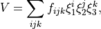
Here ‘Labels’ are the parameter names, used only for printing purposes and not in any calculations. The ‘Index’ field can be used to as a switch to indicate if the corresponding parameter was fitted or can be fitted. Otherwise it has no impact on any evaluations of the PEF values. ‘Values’ are the actual potential parameters, listed in the order implemented in the corresponding PEF POT_TYPE, for example
![\begin{split}
V(r_1,r_2,\alpha) &= f_{000} + f_{001} y_3 + f_{100} [ y_1 + y_2 ] + f_{100} [ y_1 + y_2 ] + f_{002} y_3^2 + \ldots + \\
& + b_1 e^{-g_1 r_{\rm HH}} + b_2 e^{-g_2 r_{\rm HH}^2} \\
\end{split}](_images/math/1270f549ed6ef4b0208dbfd03a3d8b0d0b79dcb1.png)
where
For the COEFF Powers option, the meaning of the columns is as follows:
Label
n1
n2
n3
n4
n5
n6
Index
Value
f000000
0
0
0
0
0
0
1
0.00000000000000E+00
f100000
1
0
0
0
0
0
1
0.00000000000000E+00
f010000
0
1
0
0
0
0
1
0.00000000000000E+00
f000100
0
0
0
1
0
0
1
0.00000000000000E+00
f000001
0
0
0
0
0
1
1
0.13239727881219E+05
f000002
0
0
0
0
0
2
1
0.46279621687684E+04
f000003
0
0
0
0
0
3
1
0.14394787420943E+04
where
‘Labels’ are the parameter name, for printing purposes only;
‘n1’, ‘n2’, ‘n3’, … are the ‘powers’ of an expansion term, e.g.
‘Index’ is a switch to indicate if the corresponding parameter was fitted or can be fitted, with no impact on any evaluations of the PEF values.
‘Values’ are the actual potential parameters. Their order is not important for this implementation as long as the corresponding powers are defined.

In case the definition of PEF requires also structural parameters, such as equilibrium bond lengths  , equilibrium inter-bond angles
  , Morse exponents
  etc., in the
 COEFF Powers form these parameters should be listed exactly in the order expected by the implemented of the PEF (similar to the COEFF LIST form), but with dummy “powers” columns so that their ‘values’ appear in the right column. For example:
POTEN
NPARAM  58
POT_TYPE  poten_C3_R_theta
COEFF  powers  (powers or list)
RE12          0      0      0      0     1.29397
theta0        0      0      0      0     0.000000000000E+00
f200          2      0      0      0        0.33240693
f300          3      0      0      0       -0.35060064
f400          4      0      0      0        0.22690209
f500          5      0      0      0       -0.11822982
.....
Here, RE12 and theta0 are two the equilibrium values and the three columns with 0 0 0 are given in order to parse their values using column 6.
TROVE configuration option used for PEF and KEO expansions
In the case of non-rigid reference configurations with periodicity used for representing the KEO and PEF as expansions, it is not uncommon that the numerically generated expansion parameter  on a grid of
  have discontinuities. They appear because of numerical problems at points like 180, 360, 720
  , i.e where trigonometric functions can change their values because of their periodicity constraints. In principle, these problems indicate that there are implementation in the code that could not be resolved. As ad hoc solution, TROVE can check and iron-out possible discontinuities by interpolating between points were the behaviour is nice and smooth. TROVE will always check and report if there are any discontinuity issues at the expansion stage, e.g.
check_field_smoothness: potencheck_field_smoothness: potencheck_field_smoothness: poten; an outlier found for iterm = 18 at i = 400: -0.46876607222E+07 vs 0.28075523334E+05
In order to switch on the “ironing-out” procedure, the iron-out card must be added anywhere in the main body of the TROVE input:
IRON-OUT
Implemented PEFs
XY2 type
There are several PEFs available for this molecule type.
POTEN_XY2_MORBID
This form is given by
![\begin{split}
V(r_1,r_2,\alpha) &= f_{000} + f_{001} y_3 + f_{002} y_3^2 + f_{003} y_4 + \ldots \\
& + (f_{100} + f_{101} y_3 + f_{102} y_3^2 + f_{103} y_4 + \ldots) [y_1 + y_2] \\
& + (f_{200} + f_{201} y_3 + f_{202} y_3^2 + f_{203} y_4 + \ldots) [y_1^2 + y_2^2] \\
& + (f_{110} + f_{111} y_3 + f_{112} y_3^2 + f_{113} y_4 + \ldots) y_1y_2 \\
& + \ldots \\
& + b_1 e^{-g_1 r_{\rm HH}} + b_2 e^{-g_2 r_{\rm HH}^2} \\
\end{split}](_images/math/97de88a0dff074ee7fedfc5b5931a99ffa464646.png)
where
For an example, see SO2_morbid_step1.inp where this PES is used.
POTEN_XY2_MORSE_COS
For description and example see ‘Potential Block’ above with the input file example for SiH2 SiH2_XY2_MORSE_COS_step1.inp. This PES was used in [21ClYu] .
POTEN_XY2_TYUTEREV
POTEN_XY2_TYUTEREV is the essentially the same PES as POTEN_XY2_MORSE_COS, with the difference that the POTEN input part does not contain the structural parameters:
POTENTIAL
NPARAM  99
POT_TYPE  poten_xy2_tyuterev
COEFF  list
b1        0    0.80000000000000E+06
b2        0    0.80000000000000E+05
g1        0    0.13000000000000E+02
g2        0    0.55000000000000E+01
f000      0    0.00000000000000E+00
f001      1    0.25298724728304E+01
f100      1    0.76001446034650E+01
...
end
Using the structural parameters in the POTEN section is important for PES refinements, see the corresponding section for details.
The input file example is h2s_step1.inp .
poten_co2_ames1
An empirical PES of CO2 is from [17HuScFr]. The input file example is CO2_bisect_xyz_step1.inp where this PES is used.
It is programmed using the powers format as follows:
POTEN
NPARAM  234
POT_TYPE  poten_co2_ames1
COEFF  powers  (powers or list)
r12ref    0 0 0  1    1.16139973893
alpha2    0 0 0  1    1.0000000000
De1       0 0 0  1    155000.0000
De2       0 0 0  1    40000.0000
Ae1       0 0 0  1   40000.0000
Ae2       0 0 0  1   20000.0000
edamp2    0 0 0  1   -2.0000
edamp4    0 0 0  1   -4.0000
edamp5    0 0 0  1   -0.2500
edamp6    0 0 0  1   -0.5000
Emin      0 0 0  1  -0.000872131085d0
Rmin      0 0 0  1  0.1161287540428520D+01
rminbohr  0 0 0  1  0.2194515245360671D+01
alpha     0 0 0  1  1.00000000000000000000
rref      0 0 0  1  1.1613997389
f000    0    0    0  0    0.3219238090183E+01
f001    0    0    1  0   -0.2181831901567E+02
f002    0    0    2  0    0.7355163655139E+02
f003    0    0    3  0   -0.1531231748456E+03
f004    0    0    4  0    0.2090079612238E+03
f005    0    0    5  0   -0.1883325770080E+03
......
end
The first part contains some structural parameters with ‘powers’ indexes filled with dummy zeros to maintain the powers format.
POTEN_XYZ_MORSE_COS_MEP
POTEN_XYZ_MORSE_FOURIER_MEP
POTEN_XY2_DMBE
POTEN_H2O_BUBUKINA
POTEN_SO2_PES_8D
POTEN_XY2_TYUTEREV_DAMP
POTEN_C3_MLADENOVIC
POTEN_C3_R_THETA
POTEN_O3_OLEG
POTEN_XY2_MLT_CO2
XYZ type
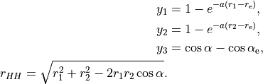
POTEN_XYZ_KOPUT
The PEF is given by (see [22OwMiYu])
The vibrational coordinates are
where  and
and  are the internal stretching coordinates and
  is the interbond angle, and the equilibrium parameters are
  ,
,  and
and  . Note that the exponent
  associated with the bending coordinate
  assumes only even values because of the symmetry of the XYZ molecule.
The input file example is CaOH_Koput_step1.inp where this PES is used.
POTEN_XYZ_TYUTEREV_SINRHO
This expansion is similar to POTEN_XY2_TYUTEREV but with the  instead of
  :
:
where
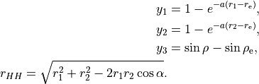
where  . The
. The potential block for NNO is illustrated below
POTEN
compact
POT_TYPE  POTEN_XYZ_TYUTEREV_SINRHO
COEFF  list
RE12          0.11282020845500E+01
RE32          0.11845554074200E+01
ALPHAE        0.18000000000000E+03
AA1           0.27742521800000E+01
AA3           0.11000000000000E+01
B1            0.50000000000000E+06
B2            0.50000000000000E+05
G1            0.15000000000000E+02
G2            0.10000000000000E+02
V0            0.54849195576882E+00
F_0_0_1       0.00000000000000E+00
F_1_0_0       0.23128656428427E+02
F_0_1_0      -0.10015174180097E+02
F_0_0_2       0.16660757971566E+05
ZXY2 type
poten_zxy2_morse_cos
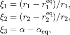
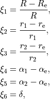
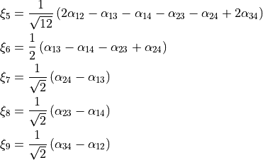
The PEF is expressed analytically as (see [15AlOvPo], [23MeOwTe])
The vibrational coordinates are
![\begin{split}
\xi_i &= 1 - \exp[-b_i(r_i-r_i^{\rm e})],\quad i={\rm 0, 1, 2}, \\
\xi_4 &= \alpha_1-\alpha_{\rm e}, \\
\xi_5 &= \alpha_2-\alpha_{\rm e}, \\
\xi_6 &= 1+\cos\tau.
\end{split}](_images/math/153bb2ee353df8aa9bd569bea428900ea03feb3f.png)
where  are the expansion parameters. Here,
  ,
,  and
and  are the bond lengths,
  and
and  are the bond angles,
  is the dihedral angle between two bond planes, and
  is a Morse-oscillator parameter.
The expansion has a symmetry adapted form, which is invariant upon interchanging the two equivalent atoms Y1 and Y2`, i.e. for  simultaneously with
  .
.
The TROVE function for this PEF is MLpoten_zxy2_morse_cos, which can be found in the module mol_zxy2.f09.
poten_zxy2_morse_cos uses the powers form for the potential parameters. An input file example for H2CS is H2CS_zxy2_morse_cos_step1.inp where this PES is used.
XY3 type (pyramidal)
POTEN_XY3_MORBID_10
This PEF is for ammonia (non-rigid) molecules with an umbrella coordinate representing the 1D inversion motion and other 5 are displacements from their equilibrium values, but it can be equally used for rigid molecules like phosphine as well. As all PEFs in TROVE, POTEN_XY3_MORBID_10 is a symmetry adapted to be fully symmetric for all operations (permutations) of the D3h(M) (and also C3v(M)) molecular group symmetry. It uses the following coordinates
![\begin{split}
\xi_i &= 1 - \exp[-a(r_i-r_i^{\rm e})],\quad i={\rm 1, 2, 3}, \\
\xi_4 &= \frac{\sqrt{2}}{\sqrt{3}} (2\alpha_1-\alpha_2-\alpha_3), \\
\xi_5 &= \frac{\sqrt{2}}{2} (\alpha_2-\alpha_3), \\
\xi_6 &= \sin\rho_{\rm e}-\sin\rho,
\end{split}](_images/math/34888a54883c6017deaf7818a4805f4da5904e0f.png)
where  (
( ) are three bond lengths,
  () are three bond angles with opposite to and
  is an umbrella coordinate defined as an ‘average’ angle between three bonds and an average symmetry axis as follows:
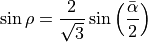
and
The corresponding Fortran function is MLpoten_xy3_morbid_10, which can found in mol_xy3.f90. It uses the Coeffs LIST form. A TROVE input example for NH3 is NH3_BYTe_step1.inp , see [09YuBaYa] where this empirical PES was used to compute the BYTe line list for ammonia.
POTEN_XY3_MORBID_11
This is a similar PES to POTEN_XY3_MORBID_10, but with the structural parameters (, and (Morse parameter)) included into the POTENTIAL block:
POTEN
NPARAM   307
POT_TYPE  poten_xy3_morbid_11
COEFF  list
 re           0  0.97580369000000E+00
 alphae       0  0.11195131680000E+03
 beta         0  0.21500000000000E+01
 VE           0  0.00000000000000E+00
 FA1          1  0.19897404278336E+02
 FA2          1  0.34574086467373E+06
 FA3          1 -0.45576605893993E+06
 FA4          1  0.21457903182324E+07
 .....
end
The Fortran function is MLpoten_xy3_morbid_11, which can found in mol_xy3.f90. A TROVE input example for H3O+ is 1H3-16O_p__eXeL__model-TROVE.inp from [20YuTeMi] , where it was used to compute an ExoMol line list for this molecule.
POTEN_XY3_MLT
POTEN_XY3_HSL
POTEN_XY3_D3H
POTEN_XY3_SEARS
POTEN_OH3P_MEP
A chain molecule of HOOH type
POTEN_H2O2_KOPUT_UNIQUE
The HOOH PES is given by the expansion
in terms of the following coordinates:
where  are three bond lengths, (
 ) are two bond angles with and
  is a dihedral angle.
This a powers type:
POTEN
NPARAM  166
POT_TYPE  POTEN_H2O2_KOPUT_UNIQUE
COEFF  powers  (powers or list)  (oo oh1  oh2 h1oo h2oo rho)
f000000       0  0  0  0  0  0  1  0.14557772800000E+01
f000000       0  0  0  0  0  0  1  0.96253006000000E+00
f000000       0  0  0  0  0  0  1  0.10108194717000E+03
f000000       0  0  0  0  0  0  1  0.11246000000000E+03
f000000       0  0  0  0  0  0  1  0.39611300000000E-02
f000001       0  0  0  0  0  1  1  0.48279121261621E-02
f000002       0  0  0  0  0  2  1  0.31552076592194E-02
f000003       0  0  0  0  0  3  1  0.27380895575892E-03
f000004       0  0  0  0  0  4  1  0.53200000000000E-04
.................
.................
end
The Fortran function is MLpoten_h2o2_koput_unique, which can found in mol_abcd.f90. A TROVE input example for HOOH is HOOH_step1.inp from [15AlOvYu] , where it was used to compute an ExoMol line list for this molecule.
POTEN_H2O2_KOPUT_MORSE
POTEN_H2O2_KOPUT
POTEN_C2H2_MORSE
POTEN_C2H2_STREYMILLS
POTEN_P2H2_MORSE_COS
POTEN_SOHF
ZXY2
POTEN_ZXY2_MLT
POTEN_ZXY2_ANDREY_01
POTEN_ZXY2_MEP_R_ALPHA_RHO_COEFF
POTEN_ZXY2_MORSE_COS
POTEN_H2CS_TZ1
POTEN_ZXY2_MEP_R_ALPHA_RHO_POWERS
A CH3Cl type system
poten_zxy3_sym
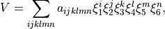
The potential function is build on the fly as follows. Taking an initial potential term of the form
(1)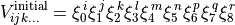
with maximum expansion order  , each symmetry operation of
  (M) is independently applied to
  , i.e.
(2)
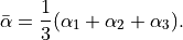
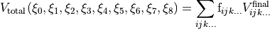
where  , to create six new terms. The results are summed together to produce a final term,
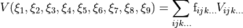
(3)
which is itself subject to the six (M) symmetry operations.  is invariant after the application of all operations and therefore the total potential function is then given by
(4)
An extract from the potential block for this PEF form is given by
POTEN
compact
POT_TYPE  poten_zxy3_sym
COEFF  powers (powers or list)
Re    0  0  0  0  0  0  0  0  0  0      1.77747221
re    0  0  0  0  0  0  0  0  0  0      1.08371647
betae 0  0  0  0  0  0  0  0  0  0    108.44534363
a0    0  0  0  0  0  0  0  0  0  0      1.65000000
b0    0  0  0  0  0  0  0  0  0  0      1.75000000
f     0  0  0  0  0  0  0  0  0  0        0.98040000
f     1  0  0  0  0  0  0  0  0  0        2.86590750
f     2  0  0  0  0  0  0  0  0  0     5526.62524810
f     3  0  0  0  0  0  0  0  0  0       92.33053568
f     4  0  0  0  0  0  0  0  0  0      347.37743030
f     5  0  0  0  0  0  0  0  0  0      190.77128084
f     6  0  0  0  0  0  0  0  0  0      105.42316955
f     0  1  0  0  0  0  0  0  0  0       19.13953554
f     0  2  0  0  0  0  0  0  0  0    22484.15160152
f     0  3  0  0  0  0  0  0  0  0    -2397.07662148
.......
.......
end
Note
For the power form of the PEF expansion, the structural (non-expansion) parameters contain dummy zeros to keep the format.
XY4
POTEN_XY4_ZZZ
POTEN_XY4_NIKITIN
POTEN_XY4_BOWMAN2000
CH:sub`2`OH
POTEN_CH3OH_REF
POTEN_CH3OH_SYM
C2H4
POTEN_C2H4_88
POTEN_C2H4_886666
C2H6
POTEN_C2H6_88
POTEN_C2H6_88_COS3TAU
C3H6
POTEN_C3H6_SYM
User-defined potentials
TROVE provide a functionality to add a new user-defined PEF without fully integrating them into the TROVE code. This is done using the general
pot_user type of Potential objects and the modules pot_user.
In the TROVE input file, a user-defined PEF will look as follows:
POTEN
POT_TYPE  general
pot_name CS2_ames1
compact
COEFF  powers  (powers or list)
r12ref    0 0 0     1.5521000000
alpha2    0 0 0     1.500000
De1       0 0 0     120000.000
De_1      0 0 0     100000.000
De3       0 0 0    160000.000
.....
.....
end
Here, general is the generic PEF type associated with a module pot_user and pot_name is an optional name of the PEF as implemented in the pot_user. The latter is a stand-along Fortran file with a unique name that must be included into the TROVE compilation set. There can be only one such file containing a pot_user module included.
A pot_user module must have the following structure:
    module pot_user
       use accuracy
       use moltype

       implicit none

       public MLdipole,MLpoten,ML_MEP,MLpoten_name

       private

       integer(ik), parameter :: verbose     = 4                          ! Verbosity level
       !
       contains
       !

      ! Check the potential name
      subroutine MLpoten_name(name)
        !
        character(len=cl),intent(in) ::  name
        character(len=cl),parameter ::  poten_name = '-NAME-'
        !
        if (poten_name/=trim(name)) then
          write(out,"('a,a,a,a')") 'Wrong Potential ',trim(name),'; should be ',trim(poten_name)
        endif
        !
        write(out,"('a')") '  Using USER-type PES ',trim(poten_name)
        !
      end subroutine MLpoten_name
      !

      recursive subroutine MLdipole(rank,ncoords,natoms,local,xyz,f)
        !
        integer(ik),intent(in) ::  rank,ncoords,natoms
        real(ark),intent(in)   ::  local(ncoords),xyz(natoms,3)
        real(ark),intent(out)  ::  f(rank)
            !
            f = user_function_defined_below(xyz)
            !
       end subroutine MLdipole

      !
      ! Defining potential energy function

      function MLpoten(ncoords,natoms,local,xyz,force) result(f)
        !
        integer(ik),intent(in) ::  ncoords,natoms
        integer(ik)            ::  i, j
        real(ark),intent(in)   ::  local(ncoords)
        real(ark),intent(in)   ::  xyz(natoms,3)
        real(ark),intent(in)   ::  force(:)
        !
        f = user_function_defined_below(xyz)
        !
      end function
       !
       function ML_MEP(dim,rho)  result(f)

        integer(ik),intent(in) ::  dim
        real(ark),intent(in)   ::  rho
        real(ark)              ::  f(dim)
        !
        f(:) = user_function_defined_below(xyz)

       end function ML_MEP

     .....
     ....

    end module pot_user
Currently, the following user-defined PEFs are available:
User-defined PEF for CH4
pot_ch4.f90
This PEF is implemented as a general (user-type) object provided in pot_ch4.f90, which is not included into the main installation and needs to be added to the TROVE compilation.
It is given by the an analytic symmetrised ( ) representation used for CH4 [14YuJe], [24YuOwTe] and SiH3 [17OwYuYa]:
where

are expanded as sum-of-products in terms of the stretch coordinates,

and symmetrized combinations of interbond angles,
where :math:a: ( ) is the Morse parameter and
  (
( ) is a reference equilibrium bond length value.
The input file (see 12C-1H4__MM__TROVE-model.inp ) has the following the powers type form:
POTEN
POT_TYPE  general
compact
COEFF  powers
re              1  0  0  0  0  0  0  0  0  0   0.10859638364000E+01
a0              2  1  0  0  0  0  0  0  0  0   0.18450000000000E+01
f000000000      3  0  0  0  0  0  0  0  0  0   0.00000000000000E+00
f100000000      4  0  0  0  0  0  0  0  0  0   0.43141069937976E+01
f000000200      5  0  0  0  0  0  0  2  0  0   0.13361306231300E+05
f000020000      6  0  0  0  0  2  0  0  0  0   0.14513674906543E+05
f000100100      7  0  0  0  1  0  0  1  0  0   0.28425912225345E+04
f011000000      8  0  1  1  0  0  0  0  0  0   0.35221935136193E+03
f020000000      9  0  2  0  0  0  0  0  0  0   0.40067820471441E+05
......
......
end
Other user-defined modules:
pot_CS2_ames1.f90
This is an Ames1 type PES by Xinchuan Huang from CS2. An example of the input poten section is as follows:
POTEN
POT_TYPE  general
pot_name CS2_ames1
compact
COEFF  powers  (powers or list)
r12ref    0 0 0     1.5521000000
alpha2    0 0 0     1.500000
De1       0 0 0     120000.000
De_1      0 0 0     100000.000
De3       0 0 0    160000.000
De_3      0 0 0     0.000
edp1      0 0 0    -0.2
edp2      0 0 0    -0.2
edp3      0 0 0    -0.5
edp4      0 0 0    -1.5
edp5      0 0 0    -0.5
edp6      0 0 0    0
Emin      0 0 0   -3.022028932409919E-006
f       0       0       0      -0.479253456996E+00
f       0       0       1      -0.513538057270E+05
f       1       0       0      -0.281216617575E+03
f       0       0       2       0.190072611427E+05
f       1       0       1      -0.372871472531E+05
f       1       1       0       0.324693877654E+05
.....
.....
end
pot_DVR3D.f90:
pot_ext_const.f90:
pot_H2O_Conway.f90:
pot_H2O_DMBE.f90:
pot_H2O_DVR3D_PES40K.f90:
pot_H3p.f90:
pot_H3p_MiZATeP.f90:
pot_HCN.f90:
pot_HCN_Harris.f90:
pot_N2O.f90:
pot_NH3_Egorov.f90
pot_NH3_Roman.f90
pot_so2.f90
pot_triatom.f90