Kinetic energy operators
There are several options for kinetic energy operators (KEO) in TROVE:
Linearised KEO: Automatically constructed KEO using the Eckart frame (rigid) or Eckart/Saywitz frame (1D non-rigid) as a Taylor expansion in terms of linearised coordinates;
Curvilinear KEO: Preprogrammed analytic KEO (exact or non-exact) using curvilinear (valence) coordinates and different frames;
External Numerical Taylor-type KEO: Externally generated KEO as a Taylor-type numerical expansion in terms of any user-defined coordinates;
External sum-of-products KEO: Externally generated KEO as a generic sum-of-products expansion via the TROVE KEO builder.
Linearised KEO
This is a standard KEO constructed using a general black-boxed algorithm applicable for an arbitrary polyatomic molecule. It has been introduced in the original TROVE paper [TROVE] and also explained in Theory. For the following, it useful to recall that TROVE uses Z-matrix curvilinear coordinates to define the linearised coordinates for a given molecule and selected frame.
Linearised KEO is a default option in TROVE. It requires the following components to be present in the TROVE code:
Coordinate transformation (
TRANSFORM) between the Z-matrix curvilinear coordinates and the target curvilinear coordinates
  used to generate the linearised coordinates
  . For example, for the Z-matrix used for NH3 (see Molecules):
ZMAT
    N   0  0  0  0  14.00307401
    H1  1  0  0  0   1.00782503223
    H2  1  2  0  0   1.00782503223
    H3  1  2  3  1   1.00782503223
end
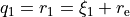
the Z-matrix coordinates are the three bond lengths  ,
,  and
and  and three bond angles
  ,
,  and
and  . The target
  curvilinear coordinates for the scheme (
TRANSFORM) r-s-delta are
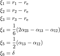
where  , where
  is the angle between the trisector and any of the bond vectors. The five linearised coordinates for a non-rigid reference configuration around
  are constructed by linearising .
Equilibrium or non-rigid reference structure associated with the frame (
Frame) and/or coordinate transformation (TRANSFORM). For NH3, a non-rigid reference frame associated with the coordinatesr-s-deltais given by (in the centre-of-mass principle axis system):
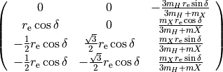
where is evaluated in a grid ![\delta_i = [-\delta_b \ldots \delta_b]](_images/math/3666a11f876dc5854f91d387861052f038e91d62.png) .
.
For the XY3 type (MOLTYPE XY3), the equilibrium structures are implemented as the subroutine ML_b0_XY3.f90 as part of the module mol_xy3.f90.
The internal coordinates type needs to be set to linear (linearised).
Consider a KEO in the general form:
(1)![\begin{split}
\hat{T}
&= \frac{1}{2} \, \sum_{\alpha=x,y,z} \; \; \sum_{\alpha^\prime=x,y,z} \hat{J}_{\alpha}\, G_{\alpha,\alpha^\prime}(\xi)\, \hat{J}_{\alpha^\prime} \\
&+ \, \sum_{\alpha=x,y,z}\;\; \sum_{n=1}^{3N-6} \left[
\hat{J}_{\alpha}\, G_{\alpha,\lambda}(\xi)\, \hat{p}_\lambda +
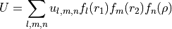
\hat{p}_\lambda \, G_{\alpha,\lambda}(\xi)\, \hat{J}_{\alpha} \right] \\
&+ \, \sum_{\lambda=1}^{M}\; \sum_{\lambda^\prime=1}^{M}
\hat{p}_\lambda \, G_{\lambda,\lambda'}(\xi)\, \hat{p}_{\lambda'} + U(\xi),
\end{split}](_images/math/870b95ebd835b74803fd943ec4afcf99cba4c206.png)
Each term in the linearised KEO is represented by a Taylor expansion in terms of  (or some 1D functions of them) around the (non-) rigid reference configuration, e.g.
(2)
where the subscript ‘lin’ is omitted for compactness. This is a sum-of-products form which simplifies the integration with the basis functions.
Analytic curvilinear KEO
A number of analytic curvilinear KEOs are available (see Frames and vibrational coordinates) and associated with the card kinetic_type as part of the KINETIC section, e.g.:
KINETIC
  kinetic_type  KINETIC_XYZ_EKE_bisect
END
Non-rigid quasi-linear triatomic molecules’s KEOs
The non-rigid quasi-linear KEOs for triatomic molecules implemented in TROVE include:
|
|
basis set |
frames/ |
BASIS expansion |
XY2 |
|
|
|
|
XY2 |
|
|
|
|
XYZ |
|
|
|
|
XYZ |
|
|
|
|
XYZ |
|
|
|
|
XYZ |
|
|
|
|
These are included in the module kin_xy2.f90.
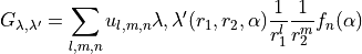
All these analytic KEO are given in a sum-of-products of 1D terms, i.e. similar to the linearised type:
for the KEO coordinates chosen as , and . Once all the matrix elements of  ,
,  and
and  are computed, the same TROVE pipeline can be used for any types of coordinates, regardless of if they are linearised or curvilinear.
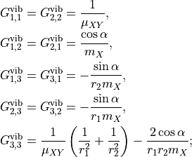
In the case of analytic XYZ and XY2 KEOs from Table %s above, the corresponding KEO terms  or pseudo-potential function
  depend on and as inverse expressions,
  ,
,  ,
,  ,
,  and
and  . We therefore represent them as sum-of-products expansions in terms of these 1D functions around the non-rigid configuration along the angle :
(3)
For example:
These KEOs become singular at the linear geometry. This is resolved by combining them with special basis set functions that exactly cancel these singularities. Such special basis functions linked to the corresponding KEOs include: laguerre-k and sinrho-laguerre-k as listed in the table above.
Moreover, the type of the 1D expansion (basic) terms in Eq. (3) should be set in the basis block for the appropriate mode. The expansion form in terms of and are called rational. Here is an example of the basis block associated with the KEO type KINETIC_XYZ_EKE_bisect:
BASIS
  0,'JKtau', Jrot 0, krot  18
  1,'numerov','rational', 'morse',  range 0,20, r 8, resc 3.0, points   2000, borders -0.3,0.90
  2,'numerov','rational', 'morse',  range 0,36, r 8, resc 1.5, points   3000, borders -0.4,0.90
  3,'laguerre-k','linear','linear', range 0,48, r 8, resc 1.0, points  12000, borders  0.,120.0 deg
END
where the 3rd card rational in the lines 1 and 2 indicate that the KEO is expanded in terms of and . Other related cards include:
KinOrder  2
TRANSFORM    R-RHO-Z-M2-M3-BISECT
MOLTYPE      XY2
REFER-CONF   non-RIGID

KINETIC
  kinetic_type  KINETIC_XYZ_EKE_bisect
END
where KinOrder 2 tells TROVE to expand the KEO and up to the 2nd order.
For intensity calculations, it is also important to link these KEO to the appropriate frame. This is because the dipole moment vectors representations strongly depend on the molecular coordinate system. In the table above, the appropriate frames (TRANSFORM) are also listed.
Analytic KEOs for rigid non-linear triatomic molecules
|
|
basis set |
frames |
|
|
XY2 |
|
|
|
|
|
It is included in the module kin_xy2.f90.
The following sum-of-products expansion is assumed:
(4)
where is one of the basic-functions types.
The KEO type KINETIC_XY2_EKE_BISECT_COMPACT_RIGID is explained in detail in basic_functions_example.rst.
How to use analytic KEOs
1. Define the KEO type using the kinetic block:
KINETIC
  kinetic_type  KINETIC_XYZ_EKE_bisect
END
2. Set the Coords type to local, KEO expansion to 2, choose the appropriate frame/and coordinates and molecule type, set the reference configuration to non-rigid:
KinOrder  2
COORDS local (curvilinear)
TRANSFORM   R-RHO-Z-M2-M3-BISECT (FRAME)
MOLTYPE XY2
REFER-CONF NON-RIGID
3. Choose appropriate basis set configuration, i.e. the KEO expansion type (e.g. rational) and the non-rigid basis set type (e.g. laguerre-k):
BASIS
  0,'JKtau', Jrot 0, krot  18
  1,'numerov','rational', 'morse',  range 0,20, r 8, resc 3.0, points   2000, borders -0.3,0.90
  2,'numerov','rational', 'morse',  range 0,36, r 8, resc 1.5, points   3000, borders -0.4,0.90
  3,'laguerre-k','linear','linear', range 0,48, r 8, resc 1.0, points  12000, borders  0.,120.0 deg
END
KEO using “basic-functions”
basic-function
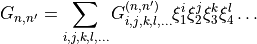
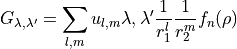
We now generalise the sum-of-products form of the KEO using the concept of “basic-functions”. Let us assume the following generalise sum-of-products form for a given KEO term  (or ) from Eq. (1):
(5)
where we introduced  as a notation for the internal valence coordinates or their combinations used to represent an exact KEO. Here,
  is a 1D generic function of a vibrational coordinate . It should be noted, that a typical internal coordinate in TROVE is a displacement from an equilibrium, e.g.
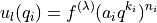
For example, for the Taylor expansion in Eq. (2), the basis-functions are
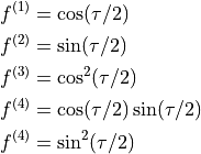
In the example from the exact KEO of the quasi-linear molecule from Eq.  , the basic functions are

In the following, we use the concept of “basic-functions” to introduce externally generated KEOs into the TROVE pipeline.
External Numerical Taylor-type KEO using “basic-functions”
As was mentioned above, TROVE can work with any ro-vibrational KEOs as long as they are represented as sum-of-products of 1D functions of vibrational coordinates. It is possible to input any externally constructed (non-singular) KEO and to be used with the TROVE pipeline. One of the most robust methods is to use the TROVE checkpoints functionality. Therefore, kinetic.chk can be used to input externally constructed KEOs in a numerical form, providing that the format (line and column orders, numbering) is preserved.
Once produced by TROVE, KEO can be saved in an ascii file in a form of expansion coefficients, which fully define it. The structure of the kinetic.chk is explained in Checkpoints.
An example of externally constructed exact KEO for the H2CS molecule using Mathematica can be found in [23MeOwTe] (both as analytic formulas and a Mathematica .nb script), where it was used with TROVE to compute an ExoMol line list. It is given using the “basic-functions” form as given by
(6)
This coordinates type (TRANSFORM) and associated frame is R-THETA-TAU (see Molecules).
The Mathemtica script Supp_Info_kinetic_energy_generator_h2cs_paper.nb (see supplementary to [23MeOwTe]) was used to produce the kinetic.chk in a numerical format using these coordinates in a rigid configuration. This can be best explained by a example, see the TROVE input at MOTY spectroscopic model.
Let us start with the basis set block:
BASIS
  0,'JKtau', Jrot 0
  1,'numerov','BOND-LENGTH', 'morse',  range 0,17, resc 1.0, points 1000, borders -0.35,1.00
  2,'numerov','BOND-LENGTH', 'morse',  range 0, 7, resc 2.0, points 1000, borders -0.5,0.9
  2,'numerov','BOND-LENGTH', 'morse',  range 0, 7, resc 2.0, points 1000, borders -0.5,0.9
  3,'numerov','ANGLE',       'linear', range 0,14, resc 1.0, points 1000, borders -1.2,1.2
  3,'numerov','ANGLE',       'linear', range 0,14, resc 1.0, points 1000, borders -1.2,1.2
  4,'numerov','DIHEDRAL',    'linear', range 0,14, resc 1.0, points 2000, borders -120.,  120.0 deg
END
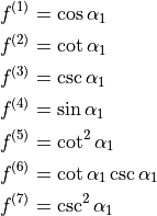
Here, the expansion types BOND-LENGTH, ANGLE and DIHEDRAL are implemented in TROVE and fully define the 1D expansion terms  in Eq. (6). In TROVE, the expansion index
  is used as an analogy for the exponent in the Taylor type expansion, Eq (2). The correlation between these indices and their actual forms are as follows.
BOND-LENGTH
Index |
Term |
0 |
1 |
1 |
|
2 |
|


ANGLE
Index |
Term |
0 |
1 |
1 |
|
2 |
|
3 |
|
4 |
|
5 |
|
6 |
|
5 |
|


DIHEDRAL
Index |
Term |
0 |
1 |
1 |
|
2 |
|
3 |
|
4 |
|
5 |
|


Other relevant input cards include:
COORDS     local
TRANSFORM  R-THETA-TAU
MOLTYPE    zxy2
REFER-CONF RIGID
The corresponding numerical KEO of H2CS in the form of the checkpoint file kinetic.chk can be also found at MOTY spectroscopic model.
Although efficient in interfacing TROVE with external KEO constructors, the latter scheme “External Numerical Taylor-type” has a few disadvantages:
The 1D basic expansion types must be implemented in TROVE, which reduces its flexibility.
When representing as sum-of-products, TROVE treats it as a Tylor-type expansion of a given order
 (defined with
 KinOrder). The number of expansion terms grows very quickly with the varying of the expansion types. In the case of the H2CS , the formal expansion order of the KEO terms in Eq. (6) (KinOrder) was 15 (i.e.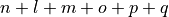 ). This was necessary to incorporate all the terms in the exact KEO of this molecule using the basic terms from the tables above. With this order, the number of the formal expansion terms in TROVE was 74613 (see card
 Ncoeffinkineti.chk) fr each KEO term and TROVE needed to allocated all of them, even though the actual number of non-zero terms was much smaller, only 208. That is, it is expensive. It should be noted that once inputted into the TROVE pipeline, with the sparserepresentation, TROVE will only work with 208 terms, but initially it would need to assume all 74613.
Ideally, we would like to have a similar functionality of the “External Numerical Taylor-type”, but with more flexibility in constructing KEO and also in the way it is inputted. In response to these requirements, the BASIC-FUNCTION feature has been introduced.
Basic-Function: External sum-of-products KEO of general type
Let us now formalise the “basic-functions” concept by representing the 1D basic functions  in Eq. (5) in the following generic form:
where  is a predefined 1D analytic form implemented in TROVE. This form allows user to formalise a generic KEO by defining it in the input file and associated kinetic.chk. To this end, the
 BASIC-FUNCTION builder is used.
As an illustration, let us consider the H2CS example and reconstruct its KEO using the BASIC-FUNCTION feature.
BASIC-FUNCTION is a TROVE block defining the shape of the KEO expansions in Eq. (6) as follows. Using the same example of H2CS, we now introduce the basic coordinates using the following constructor:
BASIC-FUNCTION
Mode 1 2
1 1 -1 I 1 1
2 1 -2 I 1 1
Mode 2 2
1 1 -1 I 1 1
2 1 -2 I 1 1
Mode 3 2
1 1 -1 I 1 1
2 1 -2 I 1 1
Mode 4 7
1 1 1 Cos 1 1
2 1 1 Cot 1 1
3 1 1 Csc 1 1
4 1 1 Sin 1 1
5 1 2 Cot 1 1
6 2 1 Cot 1 1 1 Csc 1 1
7 1 2 Csc 1 1
Mode 5 7
1 1 1 Cos 1 1
2 1 1 Cot 1 1
3 1 1 Csc 1 1
4 1 1 Sin 1 1
5 1 2 Cot 1 1
6 2 1 Cot 1 1 1 Csc 1 1
7 1 2 Csc 1 1
Mode 6 5
1 1 1 Cos 0.5 1
2 1 1 Sin 0.5 1
3 1 2 Cos 0.5 1
4 2 1 Cos 0.5 1 1 Sin 0.5 1
5 1 2 Sin 0.5 1
END
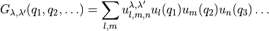
We assume that each 1D contributing term  for a given mode in the expansion of Eq. (6) can be represented using the following general form:

The basis functions can be combined together as a product to form a composed expansion type, e.g.

For example, for mode 1 (), two expansion types are selected:  and
and  , which are summarised in the following table:
mode |
|
||||
|
1 |
2 |
|||
# |
|
|
type |
|
|
1 |
1 |
-1 |
I |
1 |
1 |
2 |
1 |
-2 |
I |
1 |
1 |


Here I indicates the simple “identity” function of , i.e.

For mode 4 ( ) however 7 basic functions are used:
which is summarised in the following table:
mode |
|
||||||||
|
4 |
7 |
|||||||
# |
|
|
type |
|
|
|
type |
|
|
1 |
1 |
1 |
Cos |
1 |
1 |
||||
2 |
1 |
1 |
Cot |
1 |
1 |
||||
3 |
1 |
1 |
Csc |
1 |
1 |
||||
4 |
1 |
1 |
Sin |
1 |
1 |
||||
5 |
1 |
2 |
Cot |
1 |
1 |
||||
6 |
2 |
1 |
Cot |
1 |
1 |
1 |
Csc |
1 |
1 |
7 |
1 |
2 |
Csc |
1 |
1 |
||||


And for the last mode 6 ( ), the basic coordinates
which is summarised in the following table:
mode |
|
||||||||
|
6 |
5 |
|||||||
# |
|
|
type |
|
|
|
type |
|
|
1 |
1 |
1 |
Cos |
0.5 |
1 |
||||
2 |
1 |
1 |
Sin |
0.5 |
1 |
||||
3 |
1 |
1 |
Cos |
0.5 |
1 |
||||
4 |
1 |
2 |
Cos |
0.5 |
1 |
1 |
Sin |
0.5 |
1 |
5 |
1 |
1 |
Sin |
0.5 |
1 |
||||
Available basic function types
The following basic function types are currently available for the KEO Automatic type to be used with the BASIC-FUNCTION constructor:
# |
Keyword |
Function |
1 |
I |
|
2 |
cos |
|
3 |
sin |
|
4 |
tan |
|
5 |
csc |
|
6 |
cot |
|
7 |
csc |
|


These basic functions are associated with the BASIS expansion type automatic, see below.
Structure of kinetic.chk
For the Basic-Function feature, we use the extended format of the checkpoint file kinetic.chk, see :doc:`checkpoints. It has the following form
 0   7   93    <--- Gvib Npoints,Norder,Ncoeff
 1     1     1   0   3.86412653967     0    0    0    0    0    0
 1     2     1   0   2.80960448197     0    0    0    1    0    0
 1     3     1   0   2.80960448197     0    0    0    0    1    0
 1     4     1   0  -2.80960448197     0    1    0    4    0    0
 1     5     1   0  -2.80960448197     0    0    1    0    4    0
 1     6     1   0               0     0    0    0    0    0    0
 2     1     1   0   2.80960448197     0    0    0    1    0    0
 2     2     1   0   36.2630831225     0    0    0    0    0    0
.....
where the first three integer numbers are  ,
,  and
and  with is the number of non-zero coefficients. The columns of the main body are as follows:
----- ----- ---- --- ---------------- ---- ---- ---- ---- ----- ----
  1     2     3   4           5         6    7    8    9    10   11
----- ----- ---- --- ---------------- ---- ---- ---- ---- ----- ----
  1     1     1   0   3.86412653967     0    0    0    0    0    0
  1     2     1   0   2.80960448197     0    0    0    1    0    0
  1     3     1   0   2.80960448197     0    0    0    0    1    0
  .....
The first 5 columns are as before:
col 1: the value of the index
 in
in 
col 2: the value of the index
 in
in col 3: expansion index
 :
:
![G_{\lambda,\lambda'}^{\rm vib}(\xi) = \sum_i g_{\lambda,\lambda'}[n]\, \xi_1^{i_1} \xi_1^{i_2} \ldots \xi_{i_M}](_images/math/0b95fe996e26c2b908e9ec00593bfa80f0c7749f.png)
col 4: The non-rigid grid point
 (
( ), zero for the rigid and
col 5: Value of the expansion parameter
](_images/math/b899e1cba4f86f9f87ee00caff6da2246f17a0e5.png) .
.col 6:

col 7:

col 8:

col 9:

col 10:

col 11:
 (i.e.
(i.e.  ).
).
Special Expansion Automatic type in the basis set block
Finally, the expansion basic functions now have to be specified in the kinetic part of the basis block as the automatic type as in the following example:
BASIS
  0,'JKtau', Jrot 0
  1,'numerov','AUTOMATIC', 'morse',  range 0, 8, resc 1.0, points 1000, borders -0.35,0.9
  2,'numerov','AUTOMATIC', 'morse',  range 0, 4, resc 2.0, points 1000, borders -0.5,0.9
  2,'numerov','AUTOMATIC', 'morse',  range 0, 4, resc 2.0, points 1000, borders -0.5,0.9
  3,'numerov','AUTOMATIC', 'linear', range 0, 8, resc 1.0, points 1000, borders -1.0,1.0
  3,'numerov','AUTOMATIC', 'linear', range 0, 8, resc 1.0, points 1000, borders -1.0,1.0
  4,'numerov','AUTOMATIC', 'linear', range 0, 8, resc 1.0, points 2000, borders -120.,  120.0 deg
END
This will make sure that the correct expansion functions are used when computing KEO matrix elements.
For more on the basic functions with examples see below.
Examples for KEO Basic-functions feature