Refinement
In this chapter details will be given of the refinement procedure implemented in TROVE. Refinement in this context means to adjust the ab intio potential energy surface by comparing computed rotational-vibrational energy levels to experimental values. Parameters of the PES are varied, energy levels re-computed and compared to experiment. This process is continued until acceptable agreement between the calculated and experimental energy levels is obtained. Usually there is relatively few experimental energies and so ab intio electronic energies are used to constrain the refinement to prevent over fitting. Although experimental data is usually at fairly low energies, it is often the case that correcting the lower energy region of the PES gives more accurate values at high energies also.
Theory
Details of the method of refinement implemented in TROVE have been published [11YuBaTe] and only a brief summary will be given here. Assuming a reasonable PES has already been obtained, a correction is added in terms of internal coordinates 
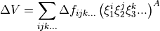
where  corresponds to totally symmetric permutation of the internal coordinates so that all symmetry properties of the molecule are properly accounted for.
  are the expansion coefficients which are found by refinement. The Hamiltonian is now given as
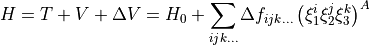
where  is the initial Hamiltonian with ab initio PES.
If the eigenvalue problem for the initial Hamiltonian has been solved,
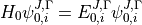
where  is the total angular momentum quantum number and
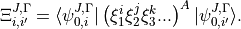
  is a symmetry label, then matrix elements of
  , using the solutions as a basis, are
where
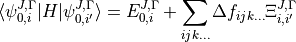
The derivatives of the energies with respect to adjustable parameters, which are required for least squares fitting, are given by the Hellman-Feynman theorem

where  and
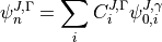
and  are eigenvalues and eigenvectors of respectively. In the J=0 representation is given by
Since TROVE typically uses linearised coordinates  to represent PESs internally, i.e. in most cases different from the analytic representation of the ab initio PES, typically given in terms of some valence coordinates
  , the TROVE eigenfunctions as well as basis functions
  are also solved and represented in terms of . Therefore, in order ro evaluate the integrals
 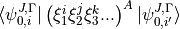 , each combination
  has to be Taylor re-expanded in terms of the linearised coordinates .
In the fittings the derivatives of the energy levels with respect to the correction parameters are evaluated at each fitting iteration in line with the standard least squares fitting Newton procedures. This is all implemented in TROVE.
Refinement with a constraint to the ab initio PES
A common problem of fitting of the model represented by a large number of parameters required for description of the full complexity of the spectroscopic model (e.g. potential energy function) is the lack of experimental data. Broadly speaking, vibrational energies are defined by the shape of the potential energy surface and are therefore controlled by the parameterised expansion of PEF, while rotational energies are defined by the equilibrium structure of a molecule via the rotational constants  ,
,  and
and  . PEFs are typically defined by a few hundreds of expansion parameters, while the experimental data does not usually cover a sufficiently large number of vibrational excited states to be probed by all the parameters required. Furthermore, not all excitations of the molecule are equally well represented in the experiment with strongest absorption bands better characterised. Overpopulated sets of potential parameters lead to an over-fitting, ill-defined or unstable minimisations an result in nonphysical potential energy functions.
To tackle the problem of correlation of the over-determined parameters, TROVE can constrain PEF to the original ab initio PES. This is implemented via a fit of the PEF (i.e. parameters representing its analytic form) simultaneously to the experimental ro-vibrational energies  for different states
  and to the ab initio potential energy data points
  at different geometries
  . In this case, the fitting functional to minimise is constructed to include the differences between the (reference) ab initio PES and the potential energy function as follows:
(1)
where  are the corresponding values of potential energy computed at the geometry and defined using the same set of potential parameters
  ;
;  is a normalised weight factor representing the relative importance of the two sets of data; and
  is the uncertainty associated with the ab initio potential energy value
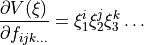
  . The required derivatives of the eigenvalues are obtained via Eqs.~eqref{e:E:finite-diff} or eqref{e:Hellmann-Feynman:2}, while the derivatives of PEF are simply
A common artifact of empirical adjustments, is that different imperfections of the model such as basis set incompleteness or approximations involved can also affect the refined PEF. As a result, these imperfections are effectively absorbed by the ‘improved’ PEF, thus making it a rather effective object that is able to reproduce the experimental energies with the accuracy achieved only with the same imperfect model used in the refinements. The ab initio constraint can provide a measure for the deformation of PEF introduced by the fit as a difference with the ab initio data. Controlling the fitting shape can be especially important when the over-fitting is difficult to avoid. Moreover, since lower fitting residuals defined by  do not necessarily mean improvement of the PEF, the deviation from the first principles data is the only objective measure of the shape of the refined PEF.
Assuming that the ab initio PES is close to the ‘’true’’ potential energy surface (in the Born-Oppenheimer approximation) within a known ab initio accuracy  , the ab initio constraint forces the refined PES also to stay close to the ab initio one. Providing that the refined PES does not deviate from the ab initio by more than , one can argue that the refined PES is at least as close to the “true” PES as the ab initio one.
How to do refinement
Setting up Refinement
The specific inputs and checkpoint files required to carry out refinement of a PES using TROVE are discussed in this section.
Prior to refinement, TROVE requires checkpoint files and eigenfunctions for the basis set being used (see above). If a calculation of the rotational-vibrational levels using an unrefined PES has already been carried out, then all necessary files for refinement will have been generated. Refinement can be carried out in the  basis.
As explained above, refinement in TROVE is represented as a correction
to the ab initio PES
an represented by refinement parameters
. In the current TROVE implementation, the refinement part
given by
While the potential is defined in the
POTENblock, the refined PES theexternalblock on the TROVE input file. This is the same structure as used to define thedipolemoment for intensity calculations and can assume a vector structure of dimension, for example in the case of DMS, the dimension is 3. For the refinement, each expansion term
externalfield is represented as a vector of dimension, where
Thus the structure of the external parameter section is just a repeat of the potential block.
..Note:: Only linear parameters like
A typical fitting
externalsection has the following form
external
dimension 102
Nparam  1
compact
TYPE  potential
COEFF   list  (powers or list)
dstep   0.005
Order   4
COORDS  morse morse linear
parameters
RE13            1.5144017558        fix
alphae          92.00507388         fix
a               0.127050746200E+01  fix
b1              0.500000000000E+06  fix
b2              0.500000000000E+05  fix
g1              0.150000000000E+02  fix
g2              0.100000000000E+02  fix
V0              0.0000000000000000
F_0_0_1     0.0              fit
F_1_0_0     0.0              fit
F_0_0_2    -0.173956405672E+05 fit
F_1_0_1     0.241119856834E+04 fit
F_1_1_0     0.0
....
end
Here
dimensionis the number of all parametersparametersandend).
Nparamtells TROVE that each component of theDIPOLEwhich can have 3 components each of which is an-dimensional analytic expansion (
) represented with
compactis the format without a fitting weight in the column before the parameter values (penultimate).
typein the case of the fitting must be potential (in the current implementation), which tells TROVE to refer to the functional type of the PEF (POT_TYPE), see Potential energy functions.
coeffis the card specifying whether that the parameters are given as alistwith predefined order as implemented in the code or via list withpowers-s (exponents). Here we use thelistform. .. Note:: AlthoughCoordsinexternaldoes not have to coincide with that inPOTEN, it is advised to used the same type in both fields for consistency.
dstepdefines the derivation step size used to evaluate high order derivatives with finite differences.
Orderdefines the re-expansion order of each
Coordsdefines the types of the linearised coordinates used in the re-expansion.
parametersindicates the beginning of the section with parameters.
fixandfitare the keywords to distinguish the parameters to fix and parameters to fit. It is important that all structural parameters are marked with thefixcard. This will insure that the derivatives and expansions offitneeds to be set only to the parameters that will need t o be varied.Note
It is important to
fixall structural parameters in theexternalsection. For the example above, the potential function it is linked to has thepot_typePOTEN_XY2_MORSE_COSand is defined as follows
POTEN
NPARAM  102
POT_TYPE  POTEN_XY2_MORSE_COS
compact
COEFF  list  (powers or list)
RE13              1.5144017558
alphae            92.00507388
a                 0.127050746200E+01
b1                0.500000000000E+06
b2                0.500000000000E+05
g1                0.150000000000E+02
g2                0.100000000000E+02
V0                0.000000000000E+00
F_0_0_1           0.000000000000E+00
F_1_0_0           0.000000000000E+00
F_0_0_2           0.173956405672E+05
F_1_0_1          -0.241119856834E+04
F_1_1_0           0.223873811001E+03
...
...
end
Here, the structural parameters are  ,
,  , Morse parameter
  as well as parameters
  ,
,  ,
,  ,
,  . The must be fixed to their values when doing the re-expansion of the external part.
Here is another example, where the potential function type poten_C3_R_theta was used:
POTEN
compact
POT_TYPE  poten_C3_R_theta
COEFF  powers  (powers or list)
RE12          0      0      0     1.29397
theta0        0      0      0     0.000000000000E+00
f000          0      0      0        0.00000000
f100          1      0      0        0.00000000
f200          2      0      0        0.33240693
f300          3      0      0       -0.35060064
f400          4      0      0        0.22690209
f500          5      0      0       -0.11822982
.....
.....
end
The external field is then given by
external
dimension 60
compact
NPARAM  1
compact
type potential
order 8
coords morse morse   linear
COEFF  powers  (powers or list)
parameters
RE12          1      0      0        1.29397   fix
theta0        0      0      0        0.0000000 fix
f000          0      0      0        0.00000000 fit
f100          1      0      0        0.00000000 fit
f200          2      0      0        0.00000000 fit
f300          3      0      0        0.00000000 fit
f400          4      0      0        0.00000000 fit
f500          5      0      0        0.00000000 fit
....
....
end
The fitted potential parameters in the external section can be assumed to be zero but never actually featured until step 4, so the actual values won’t matter at steps 1,2,3.
Calculation steps
At step 1 and 2, for the external field to be processed, the control block has to include the card external:
Step 1:
Control
Step 1
external
end
Step 2:
Control
Step 2
end
See TROVE Quick start.
Step 3 does not involve any operations with the external field and therefore should be processed as usual, e.g.
Control
Step 3
J 1
end
As discussed above, the refinement procedure requires matrix elements of the Hamiltonian and so eigenfunctions for each of interest must be computed.
After step 3, in the case of the refinements, in the control block we skip step 4 (intensities) and start step 5 (fitpot), at which matrix elements of the expansion terms are computed on the final ro-vibrational eigenfunctions obtained at step 3 for the ab initio model, for all values of and all symmetries considered. A typical Step 5 control block has the following structure:
Control
  Step 5  (FITPOT)
  external  3 60
  J  0, 1, 2, 3
  symmetries 1, 2, 3, 4
end
- Here,
3-60 in the
externalis the range of the expansion terms (i.e. corresponding to the expansion parameters ) to be processed.
J card lists all values of
to be processed. Note that it is not a range but a list i.e. the parameters can appear in any combination or order. Alias Jrot.symmetries card (alias gamma) is similar to the gamma card used in step 3. It gives a list of symmetries to be processed, again, in any combination or order.
An alias for step 5 is step fitpot. At this step, checkpoint files fitpot-J-Gamma-n.chk containing all matrix elements required for each , symmetry , for each expansion parameter  are generated. Since a file is generated for each expansion parameter n, many files are generated in this step.
At step 6 (alias step refinement), the actual fits are taking place. At this step, the control block will have similar format as for step 5:
Control
  Step 6  (refinement)
  external  3 60
  J  0, 1, 2, 3
  symmetries 1, 2, 3, 4
end
or simply with Step refinement:
Control
  Step refinement
  external  3 60
  J  0, 1, 2, 3
  symmetries 1, 2, 3, 4
end
Fitting block
At step 6, additionally to the control block change, the user needs to include the fitting section. Here is an example of a fitting block used for SiH2:
FITTING
itmax   0
fit_factor     1e4
geometries     poten.dat
output         f01
robust  0.0001
lock           100
target_rms     1e-18
fit_scale      0.25
thresh_obs-calc  10
OBS_ENERGIES
    0    1    1      0.00000  0  0   0   0   1.00
    0    1    3   1978.1533   0  0   0   2   1.00
    0    1    4   2005.469    0  1   0   0   1.00
    0    1    5   2952.7      0  0   0   3   1.00
    0    1    6   2998.6      0  1   0   1   1.00
    0    1    7   3907.4      0  1   0   2   1.00
.....
end
Here
itmaxis the number of iterations of refining carried out.itmax 0means no refinement and used for one straight-through calculation for checking purposes. TROVE will carry out refinement until the number of iterations specified is reached.
fit_factoris the relative weighting for the experimental data compared to ab initio energies
geometriesis the name of the file which contains energies of an ab initio PES used in the constrained fit. This file should give geometries in the same valence coordinates as specified by the potential energy surface for the molecule of interest in TROVE followed by the ab initio energy (from MOLPRO for example) and a weighting. The format is explained below.
outputis a string which specifies the pre-fix for auxiliary output file names, .en and .pot.
robustspecifies whether Watson Robust Fit (WRF) is used, for 0.0 it is not, for 0.0001 it is. The main function of WRF is to control and remove outliers, but can be also used to adjust the weights according to the real uncertainty of the energy levels. The non-zero values also indicate how tight the robust weighting should distinguish between good and very good uncertainties. Currently, this is a trial-and-error parameter. A good staring value is about 0.0001.
lock(akaassignment) is the card specifying if the quantum numbers will be used to match the experimental and theoretical energies: zero means that assignment is not used. By default, the energies are matched using, symmetry and the running number . , and give a unique ID for all TROVE ro-vibrational energies. However experimental energies use quantum numbers as unique identifiers and thus need to be matched to the TROVE values, which must be done by manually checking the experimental and theoretical values stored in the auxiliary .en file. The disadvantage of the running state numbers as unique IDs is that they can change though the fit, which is a very common problem. If the lockvalue is not zero, TROVE will use an automatic matching using the TROVE quantum numbers and will “lock” its matching to the given state through the fit, regardless of if the running number will change. Thelockvalue is in this case is used a threshold to match the quantum numbers. For example,lock100 means that TROVE will attempt to find a QN match within 100 cm-1 from the value associated with. , and .
target_rmsis to value of the RMS error to terminate the fit when archived. In practice however, the desired RMS error is rarely achieved.
fit_scaleis the parameter used to scale down the Newton-Raphson increment by this factor.fit_scale 1means the full increment is used, while a smaller value should make the slower but more stable. It is especially useful when the parameters are strongly correlated and has the potential even to work with over-defined problems.
thresh_obs-calcis the threshold (cm-1) to exclude accidental outliers from the fit. It is a common situation that in the middle of the fit, the state assignment of the calculated energies changes from the inial description, whether it is the running or the full set of quantum numbers are used, leading to a large residual and thus driving the fit to the wrong direction. The most reasonable approach is to exclude such an outlier from the current fit on the fly, let the process finish and then worry about the re-assignment later, before the next fit. For an almost converged fit, a typicalthresh_obs-calcvalue is 2-5 cm-1. For the initial stage, a recommended value is about 10-20 cm -1.
OBS_ENERGIES is the card indicating the beginning of the list with experimental (observed) energies.
Below is an example of a list of energies as an illustration of the format.
fitting
.......
.....
OBS_ENERGIES
  0    1    1      0.00000  0  0   0   0   1.00
  0    1    3   1978.1533   0  0   0   2   1.00
  0    1    4   2005.469    0  1   0   0   1.00
  0    1    5   2952.7      0  0   0   3   1.00
  0    1    6   2998.6      0  1   0   1   1.00
  0    1    7   3907.4      0  1   0   2   1.00
  0    1    8   3923.3      0  0   2   0   1.00
  0    1    9   3976.8      0  0   0   4   1.00
  0    1   10   3997.5      0  1   1   0   1.00
  0    4    1   1992.816    0  0   1   0   1.00
  1    2    1   11.801      2  0   0   0   1.00
  1    2    2   1010.64     2  0   0   1   1.00
  ......
  ......
end
The meaning of the columns is as follows.
   .......
   OBS_ENERGIES
   ---- ---- ---  ----------- -- -- --- ---- -----
     1    2    3       4       5  6   7   8    9
   ---- ---- ---  ----------- -- -- --- ---- -----
     0    1    1      0.00000  0  0   0   0   1.00
     0    1    3   1978.1533   0  0   0   2   1.00
     0    1    4   2005.469    0  1   0   0   1.00
     0    1    5   2952.7      0  0   0   3   1.00
     0    1    6   2998.6      0  1   0   1   1.00
     0    1    7   3907.4      0  1   0   2   1.00
     0    1    8   3923.3      0  0   2   0   1.00
     0    1    9   3976.8      0  0   0   4   1.00
     0    1   10   3997.5      0  1   1   0   1.00
     0    4    1   1992.816    0  0   1   0   1.00
     1    2    1   11.801      2  0   0   0   1.00
   ---- ---- ---  ----------- -- -- --- ---- -----


- col 1: Rotational angular momentum :math:`J` (rigourous QN);
- col 2: A symmetry count :math:`\Gamma`, e.g. for 1,2,3,4 for :math:`A_1`, :math:`A_2`, :math:`B_1` and :math:`B_2`, respectively in C :sub:`2v`(M);
- col 3: A block number, i.e. a state counting number of the states with the same :math:`J`, :math:`\Gamma`, sorted by energy.
- col 4: Experimental energy term values (cm\ :sup:`-1`) relative to ZPE.
- col 5: Rotational QN :math:`K` (non rigourous), assuming the TROVE assignment.
- col 6-8: Vibrational TROVE QNs :math:`v_1`, :math:`v_2`, :math:`v_3` etc. (non rigourous), assuming  the TROVE assignment.
- col 9: Fitting weight, which is usually inverse proportional to the experimental uncertainty of the state, but can be manipulated to influence the fit.
The format of the geometry file is as illustrated in the example below:
  -----  -------- --------------- --------- --------------
    1       2           3               4         5
  -----  -------- --------------- --------- --------------
  1.520   1.520     1.570796327      0.0000     1.000000
  1.520   1.520     1.649336143      0.3255     1.000000
  1.520   1.500     1.649336143     13.7810     1.000000
  1.500   1.520     1.649336143     13.7810     1.000000
  1.520   1.500     1.570796327     18.2147     1.000000
  1.500   1.520     1.570796327     18.2147     1.000000
  1.520   1.520     1.675516082     47.3732     1.000000
  1.500   1.520     1.675516082     59.5502     1.000000
.....
- where
col 1-3: geometries in the input (usually valence) coordinates, the same as used to define the TROVE internal coordinates, in Angstrom for the bond lengths and radians for the angles for all
 vibrational degrees of freedom.
col 4: Values of the reference “ab initio” PES for each geometry (cm-1);
col 5: Fitting weights; usually estimated using the form suggested by Partridge and Schwenke, [97PaSc]
(2)
![w_i=\left(\frac{\tanh\left[-0.0006\times(\tilde{E}_i {\rm cm} - 15{\,}000)\right]+1.002002002}{2.002002002}\right)\times\frac{1}{N \tilde{E}_i^{(w)} {\rm cm}}](_images/math/69304889885b50b7d569b18746af49ddcb40a5e4.png)
Refinement Output
The refinement procedure produces three output files. A regular .out file with a prefix the same as the .inp file and two auxiliary files .pot file and .en with prefixes as determined by the name given in the output keyword in the Fitting block.
The main output file for refinement is straightforward. The input is repeated as with other TROVE output files and then some information is given about the eigenfunctions which were read in, etc. After this TROVE prints the iteration number and then a list comparing the observed to calculated energies. For example
----------------------------------------------------------------------------------------------------
|## |  N |  J | sym|      Obs.    |    Calc.   | Obs.-Calc. |   Weight |  K   vib. quanta
----------------------------------------------------------------------------------------------------
   1    1    0  A1         0.0000       0.0000       0.0000   0.38E-05  (  0) (  0  0  0)
   2    3    0  A1      1978.1533    1981.4636      -3.3103   0.38E-05  (  0) (  0  0  2)
   3    4    0  A1      2005.4690    2008.9579      -3.4889   0.38E-05  (  0) (  1  0  0)
   4    5    0  A1      2952.7000    2956.2565      -3.5565   0.38E-05  (  0) (  0  0  3)
   5    6    0  A1      2998.6000    3003.6017      -5.0017   0.38E-05  (  0) (  1  0  1)
   6    7    0  A1      3907.4000    3914.4824      -7.0824   0.38E-05  (  0) (  0  2  0)*
   7    8    0  A1      3923.3000    3930.2323      -6.9323   0.38E-05  (  0) (  0  2  0)
   8    9    0  A1      3976.8000    3982.5964      -5.7964   0.38E-05  (  0) (  1  1  0)*
   9   10    0  A1      3997.5000    4003.2424      -5.7424   0.38E-05  (  0) (  1  1  0)
  10    1    0  B2      1992.8160    1996.2817      -3.4657   0.38E-05  (  0) (  0  1  0)
- where
##is the counting number of the experimental entries;Nis the TROVE block number (counting number with and );
Jis the rotational angular momentum;
symis the irrep in the symmetry group of the molecule in question;Obs.is the experimental energy term value (cm-1);Calc.is the calculated TROVE energy term value (cm-1);Obs.-Calc.is the residual (cm-1);Weightis the fitting weight value. This is modified from the input value, first by re-normalising all experimental weights to sum to 1, then scaling wih afit_factor and then renormalising them together with the ab initio weights (see below), which iniially also normalised to 1. When the fit starts, these weights are also adjusted through the Robust Watson re-weighting procedure, which is then printed in this output at each iteration;
Kis the TROVE rotational QN;vib. quantaare the TROVE vibrational quantum numbers.
If an asterisk (*) is printed at the end of the row (as in the first row of this example) it means that TROVE has assigned the state differently to how it was labelled in the input in the Fitting block.
The energy output is followed by three blocks of the potential parameters.
The first block lists corrections to the potential parameters is as follows:
Correction to potential parameters:
RE13          0.15144017558000E+01    fix
ALPHAE        0.92005073880000E+02    fix
AA            0.12705074620000E+01    fix
B1            0.50000000000000E+06    fix
B2            0.50000000000000E+05    fix
G1            0.15000000000000E+02    fix
G2            0.10000000000000E+02    fix
V0            0.00000000000000E+00
F_0_0_1       0.00000000000000E+00    fit
F_1_0_0       0.00000000000000E+00    fit
F_0_0_2      -0.17395640567200E+05    fit
F_1_0_1       0.24111985683400E+04    fit
F_1_1_0       0.00000000000000E+00
F_2_0_0       0.00000000000000E+00
The second block lists new values for the potential parameters  at the current iteration:
Potential parameters:
RE13          0.15144017558000E+01
ALPHAE        0.92005073880000E+02
AA            0.12705074620000E+01
B1            0.50000000000000E+06
B2            0.50000000000000E+05
G1            0.15000000000000E+02
G2            0.10000000000000E+02
V0            0.00000000000000E+00
F_0_0_1       0.00000000000000E+00
F_1_0_0       0.00000000000000E+00
F_0_0_2      -0.77718868851662E-13
F_1_0_1      -0.16208272427320E-12
F_1_1_0       0.22387381100100E+03
F_2_0_0       0.38563857069600E+05
which is followed the corrections again, but with their standard errors and also rounded according to their standard error:
Potential parameters rounded in accord. with their standard errors

RE13      -1              1.51440176
ALPHAE    -1             92.00507388
AA        -1              1.27050746
B1        -1         500000.00000000
B2        -1          50000.00000000
G1        -1             15.00000000
G2        -1             10.00000000
V0         0                    0.00
F_0_0_1    1                    -18.(            11)
F_1_0_0    1                   -109.(           242)
F_0_0_2    1                 -13218.(           390)
F_1_0_1    1                   1176.(          1047)
F_1_1_0    0                    0.00
F_2_0_0    0                    0.00
F_0_0_3    0                    0.00
The standard errors in the parentheses are understood as the last figures of the value shown, e.g.  . The standard errors are computed using the diagonal elements of the correlation matrix.
The fitting iteration output is finished with a table which gives summary details on the fit for this iteration.
----------------------------------------------------------------------------------------
|  Iter  | Points | Params |    Deviat     |     ssq_ener  |    ssq_pot  | Convergence |
----------------------------------------------------------------------------------------
|      2 |   1924 |      4 |   0.46480E+02 |  0.30230E+01  |   0.289E+04 |  0.319E+00  |
----------------------------------------------------------------------------------------
This gives the statistics of the fit including both the experimental energies (ssq_ener) and the ab initio energies (ssq_pot) used to constrain the fit as well as the total weighted standard deviation (ab initio + experiment). The latter is usually less informative because of the weighted character and a large ab initio error contribution. The most informative number in this table is ssq_ener. The Obs-Calc table, tables with potential parameters and the fit statistics are then repeated for each iteration.
Auxiliary files
To help with the refinement process, two auxiliary files are created.
The .en file has a similar purpose as the Obs-Calc table in the output file but gives all calculated energies for all states calculated by TROVE. This file is very useful when matching the experimental energies to the calculated TROVE values. It is also useful for spotting and sorting out state swaps, i.e, when accidental assignment mismatches happen. It is relatively straightforward to identify which state a mismatched/replaced experimental value should be reassigned to in order to fix the match.
The .en printout generally repeats the format of the Obs-Calc table in the output:
 ----------------------------------------------------------------------------------------------------
|## |  N |  J | Sym|     Obs.    |    Calc.   | Obs.-Calc. |   Weight |    K    quanta   (Calc./Obs.)
 ----------------------------------------------------------------------------------------------------
    1    1    0  A1         0.0000       0.0000       0.0000   0.38E-05  ( A1 ;  0 ) ( A1 ;  0  0  0 )(  0  0  0  0)
    2    0    0  A1         0.0000     999.8872       0.0000   0.00E+00  ( A1 ;  0 ) ( A1 ;  0  0  1 )
    3    3    0  A1      1978.1533    1981.4636      -3.3103   0.38E-05  ( A1 ;  0 ) ( A1 ;  0  0  2 )(  0  0  0  2)
    4    4    0  A1      2005.4690    2008.9579      -3.4889   0.38E-05  ( A1 ;  0 ) ( A1 ;  1  0  0 )(  0  1  0  0)
    5    5    0  A1      2952.7000    2956.2565      -3.5565   0.38E-05  ( A1 ;  0 ) ( A1 ;  2  0  1 )(  0  0  0  3)*
with additional QNs after in the last columns. They show the “experimental” QNs, i.e. QNs from the input file. This is to help with (re-)assignment and (re)-matching. In the case the QNs do not match, am asterisk (*) is added. It is also added if the residual obs-calc is too large.
The .pot file is a ab initio counterpart of the .en file. It list ab initio PES energies with the corresponding geometries from the geometry file used for constraining the fit. The calculated PEF values are compared to the ab initio once and the differnes are printed (cm-1), together with the fitting ab initio weights.
Here is an example of a .pot file:
                                                       Ref.         Calc.        Ref.-calc     weight
1.520000000         1.520000000         1.570796327   0.0000       27.487        -27.48678   0.5661E-03
1.520000000         1.520000000         1.649336143  0.32550       26.223        -25.89790   0.5661E-03
1.520000000         1.500000000         1.649336143   13.781       40.492        -26.71074   0.5661E-03
1.500000000         1.520000000         1.649336143   13.781       40.492        -26.71074   0.5661E-03
1.520000000         1.500000000         1.570796327   18.215       46.703        -28.48839   0.5661E-03
1.500000000         1.520000000         1.570796327   18.215       46.703        -28.48839   0.5661E-03
1.520000000         1.520000000         1.675516082   47.373       72.300        -24.92634   0.5661E-03
1.500000000         1.520000000         1.675516082   59.550       85.239        -25.68921   0.5661E-03
where the first  columns (number of the vibrational degrees of freedom) list the valance coordinates as defined in the
 geometry file, followed the ab initio or “reference” (Ref.) PES values, calculated (Calc.) values, the differences Ref.-Calc. and the fitting weights (after being normalised within the ab initio set, combined with the experimental weights and re-normalised to 1 again).
Watson Robust fitting
In progress
Running Refinement
In progress