Dipole moment functions

TROVE provides a larger number of dipole moment functions (DMFs) for different molecules already implemented. Most of these PEFs are in modules pot_* contained in file pot_*.f90.

pot_xy2.f90

pot_xy3.f90

pot_zxy2.f90

pot_abcd.f90

pot_xy4.f90

pot_zxy3.f90

These are a part of the standard TROVE compilation set. Alternatively, a user-defined DMF can be included into the TROVE compilation as a generic ‘user-defined’ module pot_user.

Dipole (External) Block

The DMFs are defined in the TROVE input file using the Dipole block, which is just an alias for the external input structure. A typical Dipole input is as follows:

DIPOLE
dimension 3
NPARAM  264 0 0
compact
DMS_TYPE  XY3_SYMMB
COEFF   list
COORDS  linear linear linear linear linear linear
Order   6  6  6
dstep 0.005
parameters
charge              0.00000000
nparamA           112.00000000
RhoE               90.00000000
RE14                1.01032000
beta                1.00000000
d0                  4.56621083
f1a                -9.36438932
f2a                32.96400671
...
end

For an example, see 14N-1H3__BYTe__TROVE__step1.inp where this DMF is used.

dimension (aliases rank, dim): This is the dimension of the external field. An “external” is treated in TROVE as a vector of dimension $D$ , which in the case of dipole can be up to $D=3$ , but will depend on the implementation. This parameter is to help structure the input dipole parameters according to the dipole components, if necessary.
NPARAM is used to specify the number of parameters to define the DMF and should contain $D$ input values.
compact: is recently implemented card which switches to the “compact” format with no “fitting-indexes” column present.
DMS_TYPE (TYPE) is the name of the DMF as implemented in pot_*.f90 file and referenced in mlecules.f90.
COEFF indicates if the DFM parameters are given as a list of parameter values (LIST) or values with the corresponding expansion powers (POWERS), see example below.
COORDS: coordinate types used to re-expand the dipole field in terms of the internal TROVE coordinates.
Order: The corresponding expansion order.
dstep: finite difference step used in the re-expansion. The default value is 0.005 Ang.
parameters: card indicating the section with the dipole parameters entries specific for the given DMS_TYPE.

The dipole moment parameters are listed after the keyword parameters and terminated with the keyword END. The number of the entries should be equal exactly to the sum of NPARAM values.

For the COEFF list option, the meaning of the columns is as follows:

Label	Value
charge	0.00000000
nparamA	112.00000000
RhoE	90.00000000
RE14	1.01032000
beta	1.00000000
d0	4.56621083
f1a	-9.36438932
f2a	32.96400671

The first column with the name of the parameters, which is for clearness only. This field is only used for printing purposes and otherwise nor-referenced in the code in any way. The second column contains the actual value of the given parameter. The input is directly associated with the corresponding implementation and therefore the order is important.

An alternative, legacy, format with no compact card assumes an additional column with the so-called “fitting-indexes” indicating if the parameter was varied in the fitting to the ab initio data. Here is an example:

parameters
charge       0           0.00000000
nparamA      1          112.00000000
RhoE         0         90.00000000
RE14         0          1.01032000
beta         0          1.00000000
d0           4          4.56621083
f1a          8         -9.36438932
f2a          8         32.96400671
f3a          7        -80.82339377
....

where column 2 contains the “fitting-indexes”. These indexes are not used by TROVE. They are kept in order to simplify the interfacing between the ab initio fitting and TROVE, but can be always omitted with the help of the card compact.

Here is an example of the input format using individual expansion “powers”, COEFF powers (from CO₂):

    DIPOLE
    rank 3
    NPARAM  971 0 0
    compact
    TYPE  DIPOLE_AMES1
    COEFF   powers  (powers or list)
    COORDS  linear linear linear
    Orders   16 16 16
    threshold   1e-8
    Parameters
    re    0 0 0 0  1.15958d0
    ae    0 0 0 0  180.00
    d000    0    0    0   0      -0.4801402388843266D+00
    d001    0    0    1   0       0.1203598337496481D+00
    d002    0    0    2   0      -0.5662267278952241D-01
    d003    0    0    3   0      -0.2529381009630170D-01
    d004    0    0    4   0      -0.1271678002798687D+00
    d005    0    0    5   0       0.3033049145401118D+01
    d006    0    0    6   0      -0.1754036600894653D+02
.....
end

See the TROVE input CO2_bisect_xyz_step1.inp.

Assuming the DMF form as an expansion

$\mu_\alpha(\xi_1,\xi_2,\xi_3) = \sum_{k,j,k} d_{i,j,k} \xi_1^i \xi_2^j \xi_3^k,$

the input card has the following format

Label

$i$

$j$

$k$

Index

Value $_{i,j,k}$

d000

0

0

0

0

-0.4801402388843266D+00

d001

1

0

0

0

0.1203598337496481D+00

d002

0

1

0

0

-0.5662267278952241D-01

where

‘Labels’ are the parameter name, for printing purposes only;

$i$ , $j$ , $k$ are the ‘powers’ of an expansion term;

‘Index’ is a switch to indicate if the corresponding parameter was fitted or can be fitted, with no impact on any evaluations of the PEF values. It is not present in the compact form.

‘Values’ are the actual dipole parameters. For powers, their order is not important.

In case the definition of DMF requires also structural parameters, such as equilibrium bond lengths $r_{\rm e}$ , equilibrium inter-bond angles $\alpha_{\rm e}$ , in the COEFF Powers form these parameters should be listed exactly in the order expected by the implemented of the PEF (similar to the COEFF LIST form), but with dummy “powers” columns so that their ‘values’ appear in the right column, as in the example above, re and ae are two the equilibrium values and the three columns with 0 0 0 are given in order to parse their values using exactly column 6.

Implemented DMFs

XY₂ type

See module pot_xy2.f90.

There are several PEFs available for this molecule type.

`xy2_pq_coeff`

This is a bisector-frame DMF, given by two components, $\mu^{(q)}$ and $\mu^{(p)}$ with the $q$ axis being the bisector. The following expansions in terms of the coordinate displacements $\Delta r_1 = r_{\rm 1} - r_{\rm e}$ , $\Delta r_2 = r_2 - r_{\rm e}$ , and $\cos\rho_{\rm e} - \cos\rho$ , where $\rho = \pi - \theta$ are used, with $\theta$ is the bond angle, and $r_1$ and $r_2$ are the bond lengths:

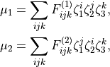
(1) $\begin{split} \mu^{(q)} (\Delta r_1, \Delta r_2, \Delta \alpha ) &= \sin\alpha \left[ \mu_0^{(q)}(\alpha) + \sum_{j} \mu_{j}^{(q)}(\alpha) \Delta r_j + \sum_{j\le k} \mu_{jk}^{(q)}(\alpha) \Delta r_j \Delta r_k \right. \\ & \left . + \sum_{j\le k \le m} \mu_{jkm}^{(q)}(\alpha) \Delta r_j \Delta r_k \Delta r_m + \sum_{j\le k \le m \le n} \mu_{jkmn}^{(q)}(\alpha) \Delta r_j \Delta r_k \Delta r_m \Delta r_n + \ldots \right], \\ \mu^{(p)} (\Delta r_1, \Delta r_2, \Delta \alpha ) &= \mu_0^{(p)}(\alpha) + \sum_{j}^{(p)} \mu_{j}^{(p)} (\alpha) \Delta r_j + \sum_{j\le k} \mu_{jk}^{(p)}(\alpha) \Delta r_j \Delta r_k \\ & + \sum_{j\le k \le m} \mu_{jkm}^{(p)}(\alpha) \Delta r_j \Delta r_k \Delta r_m + \sum_{j\le k \le m \le n} \mu_{jkmn}^{(p)}(\alpha) \Delta r_j \Delta r_k \Delta r_m \Delta r_n + \ldots , \end{split}$

where all indices $j, k, m$ , and $n$ assume the values 1 or 2,

(2) $\begin{split} \mu_{jk\ldots}^{(q)}(\alpha) =& \sum_{i=0}^{N} Q_{ij\ldots}^{(i)} (\cos\alpha_{\rm e} - \cos\alpha )^i, \\ \mu_{jk\ldots}^{(p)}(\alpha) =& \sum_{i=0}^{N} P_{ij\ldots}^{(i)} (\cos\alpha_{\rm e} - \cos\alpha )^i, \end{split}$

and the $Q_{ij\ldots}^{(i)}$ and $P_{ij\ldots}^{(i)}$ are molecular dipole parameters. The expansion coefficients in Eqs. (2) are subject to the conditions that the functions $\mu^{(q)}$ are unchanged under the interchange of the identical protons, whereas the function $\mu^{(p)}$ is antisymmetric under this operation. There are 72 and 99 paramters $Q_{ij\ldots}^{(i)}$ and $P_{ij\ldots}^{(i)}$ , respectively. An example of xy2_pq_coeff is illustrated above and can be foound in H2S_EKE_basic-functions_step1.inp.

The implementation can be found in subroutine MLdms2pqr_xy2 from the module pot_xy2.f90. The transformation between the TROVE frame and the frame of the specifc dipole of the XY₂ is perfomed in the subroutine MLloc2pqr_xy2, e.g.:

!
select case(trim(molec%frame))
   !
case('R-RHO-Z','R-RHO-Z-M2-M3','R-RHO-Z-M2-M3-BISECT','BISECT-Z')
   !
   a0(2, 1) = -r(1) * cos(alpha_2)
   a0(2, 3) = -r(1) * sin(alpha_2)
   !
   a0(3, 1) = -r(2) * cos(alpha_2)
   a0(3, 3) =  r(2) * sin(alpha_2)
case ...

`XY2_PQ_LINEAR`

This is similar to xy2_pq_coeff, but with the bending expansion in Eq. :eq:` e-muQ-exp` in terms of the displacement $\alpha-\alpha_{\rm e}$ :

(3) $\begin{split} \mu_{jk\ldots}^{(q)}(\alpha) =& \sum_{i=0}^{N} Q_{ij\ldots}^{(i)} (\alpha - \alpha_{\rm e} )^i, \\ \mu_{jk\ldots}^{(p)}(\alpha) =& \sum_{i=0}^{N} P_{ij\ldots}^{(i)} (\alpha - \alpha_{\rm e} )^i, \end{split}$

`DIPOLE_AMES1`

This DMF is of the AMES1 type represented using the point-charge molecular bond frame [14HuScLe] given by projections on the molecular bond vectors $\vec{r}_1$ and $\vec{r}_2$ :

$\vec{\mu} = \mu_x \vec{i} + \mu_z \vec{k} = \mu_1 \vec{r}_1 + \mu_2 \vec{r}_2$

where $\mu_x$ and $\mu_z$ are the TROVE frame vectors and $\mu_1$ and $\mu_2$ are the ab initio dipoles in the molecular bond frame (the $\mu_y$ component is always zero). The two point-charge dipole moment components $\mu_1$ and $\mu_2$ are represented in terms of the vibrational coordinates as

(4) $\begin{split} \zeta_1 &= r_1-r^{\rm ref}_1, \\ \zeta_2 &= r_2-r^{\rm ref}_2, \\ \zeta_3 &= \cos\alpha-1. \end{split}$

with the following analytic Taylor-type expansions used (see e.g. [14HuScLe]):

$\begin{split} \mu_1 &= \sum_{ijk} F^{(1)}_{ijk} \zeta_1^{i} \zeta_2^{j} \zeta_3^{k} , \\ \mu_2 &= \sum_{ijk} F^{(2)}_{ijk} \zeta_1^{j} \zeta_2^{i} \zeta_3^{k} , \end{split}$

As an example can be found of a system where this form was used, see CO2_bisect_xyz_step1.inp.

`DIPOLE_SO2_AMES1`

This form is essentially the same as DIPOLE_AMES1 but some specific characteristic used for the SO₂ molecule in [14HuScLe].

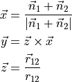
`XY2_C3_SCHROEDER`

This DMF is based on the DMF form reported by Schroeder et al. [16ScSe] for C₃. This DMF is in the Ecakrt frmame expressed in terms of two in-plane components, $\mu^{\parallel}$ and $\mu^{\perp}$ , as Taylor expansions around the equilibrium geometry:

$\begin{split} \mu^{\parallel} &= D^{\parallel}_{ijk} \Delta r_1^i \,\Delta r_2^j \, \Delta \alpha^k , \\ \mu^{\perp} &= D^{\perp}_{ijk} \Delta r_1^i \,\Delta r_2^j \, \Delta \alpha^k . \end{split}$

Since TROVE’s frame is usually different from the DMF frame (e.g. bisector) in the ro-vibrational calculations, this dipole moments functions needs to be rotated. This is done using the rotation angle $\phi$ from an equilibrium bysector frame $r_{n\alpha}^0$ to the instantaneous frame $r_{n\alpha}$ ( $n=1,2,3$ and $\alpha=x,y,z$ ) in the in the $xz$ plane as given by

$\tan\phi = \frac{m_{\rm X} ( r^0_{1,z} r_{1,x}-r^0_{1,x} r_{1,z} )+m_{{\rm Y}_1} (r^0_{2,z}r_{2,x}-r^0_{2,x}r_{2,z} )+m_{{\rm Y}_2}(r^0_{3,z}r_{3,x}-r^0_{3,x}r_{3,z}) }{ m_{\rm X} (r^0_{1,z} r_{1,z}+r^0_{1,x}r_{1,x})+m_{{\rm Y}_1}(r^0_{2,z}r_{2,z}+r^0_{2,x}r_{2,x})+m_{{\rm Y}_2}(r^0_{3,z}r_{3,z}+r^0_{3,x}r_{3,x}) }$

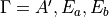
`DIPOLE_PQR_XYZ_Z-FRAME`

This is frame used to represent DMF of XYZ non-symmetri molecules with the $z$ ( $p$ ) axis along the vecror $r_1$ and other two axes defined using the following conditions:

$\begin{split} \vec{p} &= \frac{\vec{r}_1}{r_1} \\ \vec{y} &= \frac{\vec{r}_1 \times \vec{r}_2 }{|\vec{r}_1 \times \vec{r}_2|} \\ \vec{q} &= \vec{y}\times \vec{p} \end{split}$

The corrsponding components $\mu^{(q)}$ and $\mu^{(p)}$ are expanded using the same form as in Eq. (1) but with no constraints on the permutations of the atoms.

`DIPOLE_PQR_XYZ_Z-FRAME_SINRHO`

The same as DIPOLE_PQR_XYZ_Z-FRAME but with $\sin(\alpha_{\rm e}-\alpha)$ as an expansion variable in Eq. (1) instead of $\cos\alpha_{\rm e} - \cos\alpha$ :

(5) $\begin{split} \mu_{jk\ldots}^{(q)}(\alpha) =& \sum_{i=0}^{N} Q_{ij\ldots}^{(i)} (\sin(\alpha_{\rm e}-\alpha))^i, \\ \mu_{jk\ldots}^{(p)}(\alpha) =& \sum_{i=0}^{N} P_{ij\ldots}^{(i)} (\sin(\alpha_{\rm e}-\alpha))^i, \end{split}$

When $\alpha_{\rm e} = \pi$ (linear molecules), $\sin(\pi-\alpha) = \sin\rho$ , which explanes the suffix _sinrho in the name of thi DMF, wich is aimed at linear molecules.

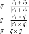
DIPOLE_PQR_XYZ

This a bisector dipole frame for the XYZ type molecules. It is defined by

$\begin{split} \vec{q} &= \frac{\vec{r}_1+\vec{r}_2}{|\vec{r}_1+\vec{r}_2|} \\ \vec{y} &= \frac{\vec{r}_1 \times \vec{q}}{|\vec{r}_1 \times \vec{q}|} \\ \vec{p} &= \vec{q}\times \vec{y} \end{split}$

The exapnsion of the dipole moment components in terms of $r_1$ , $r_2$ and $\alpha$ as in Eq. (3). See 7Li-16O-1H__OYT7__TROVE.model for an example of a TROVE input.

`DIPOLE_PQR_XYZ_Z-BOND`

Subroutine: MLdms2pqr_xyz_z_bond.

This is a generalisation of DIPOLE_PQR_XYZ_Z-FRAME, which does not make any assumtion on the frame of the original dipole, only on its expansion form given as in Eq. (3). The role of DIPOLE_PQR_XYZ_Z-BOND is to transform it to the TROVE frame, which in this case is the with the $z$ axis oriented along the bond $\vec{r}_1$ :

$\begin{split} \vec{x} &= \frac{\vec{n}_1+\vec{n}_2}{|\vec{n}_1+\vec{n}_2|} \\ \vec{y} &= \vec{z}\times \vec{x} \\ \vec{z} &= \frac{\vec{r}_{12}}{r_{12}} \end{split}$

`DIPOLE_PQR_XYZ_BISECTING`

Subroutine: MLdms2pqr_xyz_bisecting.

This is a generalisation of DIPOLE_PQR_XYZ, which does not make any assumtion on the frame of the original dipole, only on its expansion form given as in Eq. (3). The role of DIPOLE_PQR_XYZ_BISECTING is to transform it to the TROVE frame, which in this case is the with the $x$ axis oriented along the bisector:

$\begin{split} \vec{q} &= \frac{\vec{r}_1+\vec{r}_2}{|\vec{r}_1+\vec{r}_2|} \\ \vec{y} &= \frac{\vec{r}_1 \times \vec{q} }{|\vec{r}_1 \times \vec{q}|} \\ \vec{p} &= \vec{q}\times \vec{y} \end{split}$

`DIPOLE_AMES1_XYZ`

This form is a modification of DIPOLE_AMES1 for non-symmetric molecules.

As an example can be found of a system where this form was used, see 16O-12C-32S__OYT8__TROVE.model as well in OYT8 spectroscopic model, where it was used to compute an ExoMol line list for OCS [24OwYuTe].

`XY2_SCHROEDER_XYZ_ECKART`

This is an XYZ version of the XY2_C3_SCHROEDER type.

DIPOLE_H2O_LPT2011

DMF from [11LoTePo]. It is included into subroutine MLdipole_h2o_lpt2011 in prop_xy2.f90.

DIPOLE_PQR_XYZ_Z-BOND

DIPOLE_PQR_XYZ_BISECTING`

DIPOLE_BISECT_S1S2T_XYZ

XY2_QMOM_SYM

XY2_ALPHA_SYM

XY2_QMOM_BISECT_FRAME

TEST_XY2_QMOM_BISECT_FRAME

XY2_SR-BISECT-NONLIN

TEST_XY2_SR-BISECT-NONLIN

XY3

See module pot_xy3.f90.

XY3_MB

This DMF is implemented as a subroutine MLdms2xyz_xy3_mb and was reported in [06YuCaTh]. This form was used to produce a line list for PH₃ in [13SoYuTe]. An input example is in 31P-1H3__SAlTY__TROVE.model and can be also found at https://exomol.com/models/PH3/31P-1H3/SAlTY/.

Consider the $r_i$ as the instantaneous value of the distance between X and Y $_i$ , where Y $_i$ is the nucleus labeled $i$ (= 1, 2, or 3); $\alpha_i$ denotes the bond angle $\angle$ (Y $_j$ XY $_k$ ) where $(i,j,k)$ is a permutation of the numbers (1,2,3).

We utilize the so-called Molecular-Bond (MB) representation to describe the $r_i$ and $\alpha_j$ dependence of the electronically averaged dipole moment vector $\bar{\bf \mu}$ for XY₃. In the MB representation it is given by

(6) $\bar{\bf \mu} = \bar{\mu}_1^{\rm Bond}\, \vec{\bf e_1} + \bar{\mu}_2^{\rm Bond}\, \vec{\bf e_2} + \bar{\mu}_3^{\rm Bond}\, \vec{\bf e_3}$

where the three functions $\bar{\mu}_i^{\rm Bond}$ , $i$ $=$ 1, 2, 3, depend on the vibrational coordinates, and $\vec{\bf e}_i$ is the unit vector along bond $i$ ,

$\vec{\bf e}_i = \frac{\vec{\bf r}_i-\vec{\bf r}_4}{|\vec{\bf r}_i-\vec{\bf r}_4|}$

with $\vec{\bf r}_i$ ( $i$ $=$ 1, 2, 3) as the position vector of proton $i$ and $\vec{\bf r}_4$ as the position vector of X. The representation of $\bar{\bf \mu}$ in Eq. (6) is “body-fixed” in the sense that it relates the dipole moment vector directly to the instantaneous positions of the nuclei (i.e., to the vectors $\vec{\bf r}_i$ ).

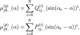
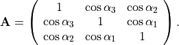
Following [06YuCaTh], we express the three functions $\bar{\mu}_i^{\rm Bond}$ , $i$ $=$ 1, 2, 3, as

(7) $\bar{\mu}_i^{\rm Bond} = \sum_{j=1}^3 \left({\mathbf A}^{-1} \right)_{ij} \, \left( \bar{\bf \mu} \cdot \vec{\bf e}_j \right)$

where $({\mathbf A}^{-1} )_{ij}$ is an element of the non-orthogonal $3 \times 3$ matrix ${\mathbf A}^{-1}$ obtained as the inversefootnote% {When the molecule is planar, the determinant $\vert \mathbf A \vert$ $=$ 0 and $\mathbf A$ cannot be inverted. In this case we set $\bar{\mu}_3^{\rm Bond}$ $=$ 0 in Eq. (6) and express $\bar{\bf \mu}$ in terms of $\vec{\bf e}_1$ and $\vec{\bf e}_2$ only, i.e., we determine $\bar{\mu}_1^{\rm Bond}$ and $\bar{\mu}_2^{\rm Bond}$ in terms of $\bar{\bf \mu} \cdot \vec{\bf e}_1$ and $\bar{\bf \mu} \cdot \vec{\bf e}_2$ .} of

${\mathbf A} = \left( \begin{array}{ccc} 1 & \cos\alpha_3 & \cos\alpha_2 \\ \cos\alpha_3 & 1 & \cos\alpha_1 \\ \cos\alpha_2 & \cos\alpha_1 & 1 \end{array} \right)\hbox{.}$

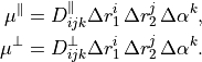
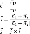
For symmetry reasons, all three projections can be expressed in terms of a single function $\mu_0(r_1,r_2,r_3,\alpha_1,\alpha_2,\alpha_3)$ :

$\begin{split} \bar{\bf \mu} \cdot \vec{\bf e}_1 &= \mu_0(r_1,r_2,r_3,\alpha_1,\alpha_2,\alpha_3) = \mu_0(r_1,r_3,r_2,\alpha_1,\alpha_3,\alpha_2), \\ \bar{\bf \mu} \cdot \vec{\bf e}_2 &= \mu_0(r_2,r_3,r_1,\alpha_2,\alpha_3,\alpha_1) = \mu_0(r_2,r_1,r_3,\alpha_2,\alpha_1,\alpha_3), \\ \bar{\bf \mu} \cdot \vec{\bf e}_3 &= \mu_0(r_3,r_1,r_2,\alpha_3,\alpha_1,\alpha_2) = \mu_0(r_3,r_2,r_1,\alpha_3,\alpha_2,\alpha_1), \end{split}$

and this function is chosen as an expansion

(8) $\begin{split} \mu_0 = \mu_{0 }^{(0)} + \sum_{k} \mu_{k }^{(0)} \xi_k + \sum_{k,l} \mu_{k l }^{(0)} \xi_k \xi_l & + \sum_{k,l,m} \mu_{k l m }^{(0)} \xi_k \xi_l \xi_m \nonumber\\ & + \sum_{k,l,m,n} \mu_{k l m n}^{(0)} \xi_k \xi_l \xi_m \xi_n + \ldots \end{split}$

in the variables

$\begin{split} \xi_k &= (r_k-r_{\rm e}) \exp \left( -\beta^2 \, (r_k-r_{\rm e})^2 \right), \;\; k=1,2,3, \\ \xi_l &= \cos \left(\alpha_{l-3}\right) - \cos \left(\alpha_{\rm e}\right) \hbox{,} \;\; l=4,5,6 \hbox{,} \end{split}$

where $r_{\rm e}$ and $\alpha_{\rm e}$ are the equilibrium values of the bond lengths and bond angles, respectively. We include the factor 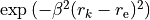$\exp \left( -\beta^2 (r_k-r_{\rm e})^2 \right)$ in order to keep the expansion from diverging at large $r_k$ .

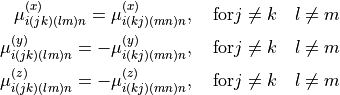
The expansion coefficients $\mu_{k,l,m,\ldots}^{(0)}$ are pairwise equal. We have

$\mu_{k',l',m', \ldots}^{(0)} = \mu_{k,l,m, \ldots}^{(0)}$

when the indices $k',l',m', \ldots$ are obtained from $k,l,m, \ldots$ by replacing all indices 2 by 3, all indices 3 by 2, all indices 5 by 6, and all indices 6 by 5.

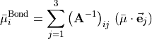
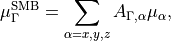
XY3_SYMMB

This form is a non-rigid analogy of XY3_MB allowing the pyrimidal molecule XY₃ to go through the planar configuration and was introduced in [09YuBaYa]. It is implemented in subroutine MLdms2xyz_xy3_symmb in pot_xy3.f90. This form has been used in several studies of non-rigid pyrimidal molecules including NH₃, CH₃, OH₃⁺.

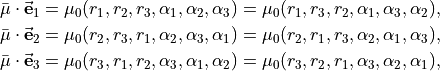
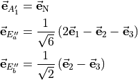
A disadvantage of the XY3_MB representation is the ambiguity at and near planar geometries when the three vectors $\vec{\bf e}_i$ become linearly dependent, or nearly linearly dependent, and singularities appear in the determination of the $\bar{\mu}_i^{\rm Bond}$ functions. This is overcome by reformulating the $\bar{\mu}_i^{\rm Bond}$ functions in terms of symmetry-adapted combinations of the MB projections $\left(\bar{\bf \mu}\cdot \vec{\bf e}_j \right)$

$\begin{split} \mu_{A''_1}^{\rm SMB}&= \left( \bar{\bf \mu} \cdot \vec{\bf e}_{\rm N} \right) \\ \mu_{E'_a}^{\rm SMB} &= \frac{1}{\sqrt{6}} \left[ 2 \left( \bar{\bf \mu} \cdot \vec{\bf e}_1 \right) - \left( \bar{\bf \mu} \cdot \vec{\bf e}_2 \right) - \left( \bar{\bf \mu} \cdot \vec{\bf e}_3 \right) \right] \\ \mu_{E'_b}^{\rm SMB} &= \frac{1}{\sqrt{2}} \left[ \left( \bar{\bf \mu} \cdot \vec{\bf e}_2 \right) - \left( \bar{\bf \mu} \cdot \vec{\bf e}_3 \right) \right], \end{split}$

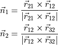
where an additional reference MB-vector $\vec{\bf e}_{\rm N} = \vec{\bf q}_{\rm N}^{}/\vert \vec{\bf q}_{\rm N}^{}\vert$ was introduced by means of the ‘trisector’

$\vec{\bf q}_{\rm N} = (\vec{\bf e}_1 \times \vec{\bf e}_2) + (\vec{\bf e}_2 \times \vec{\bf e}_3) + (\vec{\bf e}_3 \times \vec{\bf e}_1).$

This symmetrized molecular bond representation is denoted as “SMB”. The subscripts of the $\mu_{\Gamma}^{\rm SMB}$ functions ( $\Gamma = A''_1,E'_a, E'_b$ ) refer to irreducible representations of D_3h(M); $\mu_{A''_1}^{\rm SMB}$ has $A''$ symmetry in D_3h(M), and $(\mu_{E'_a}^{\rm SMB}, \mu_{E'_b}^{\rm SMB})$ transform as the $E'$ irreducible representation. The symmetrized vectors

$\begin{split} \vec{\bf e}_{A'_1} &= \vec{\bf e}_{\rm N} \\ \vec{\bf e}_{E''_a} &= \frac{1}{\sqrt{6}} \left( 2 \vec{\bf e}_1 - \vec{\bf e}_2 - \vec{\bf e}_3 \right) \\ \vec{\bf e}_{E''_b} &= \frac{1}{\sqrt{2}} \left( \vec{\bf e}_2 - \vec{\bf e}_3 \right) \end{split}$

have $A'_1$ and $E''$ symmetry in the same manner.

The dipole moment vector $\bar{\bf \mu}$ vanishes at symmetric, planar configurations of D_3h geometrical symmetry. Also, the $\mu_{A'_1}^{\rm SMB}$ component is antisymmetric under the inversion operation $E^*$ and vanishes at planarity, which leaves only two independent components of $\bar{\bf \mu}$ at planarity.

The advantage of having a DMS representation in terms of the projections $\left( \bar{\bf \mu} \cdot \vec{\bf e}_j \right)$ is that it is “body-fixed”. It relates the dipole moment vector directly to the instantaneous positions of the nuclei (i.e., to the vectors $\vec{\bf r}_i$ ). These projections are well suited to being represented as analytical functions of the vibrational coordinates. For intensity simulations, however, we require the Cartesian components $\mu_{\alpha}$ , $\alpha=x,y,z$ of the dipole moment along the molecule-fixed $xyz$ axes. These are obtained by inverting the linear equations

(9) $\mu_{\Gamma}^{\rm SMB} = \sum_{\alpha=x,y,z} A_{\Gamma,\alpha} \mu_{\alpha},$

where $A_{\Gamma,\alpha}$ , is the $\alpha$ -coordinate ( $\alpha=x,y,z$ ) of the vector $\vec{\bf e}_{\Gamma}$ ( $\Gamma=A',E_a,E_b$ ). When the molecule is planar, $\mu_{A''_1}^{\rm SMB}$ is zero, as is the corresponding right-hand side in Eq. (9). Thus, at planar configurations the system of linear equations in $\mu_{\alpha}$ contains two non-trivial equations only. At near-planar configurations $\mu_{A''_1}^{\rm SMB}$ is not exactly zero and cannot be neglected, and so Eq. (9) becomes near-linear-dependent. The symmetry-adapted representation of $\mu^{\rm SMB}$ appears to be well defined even for these geometries.

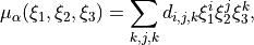
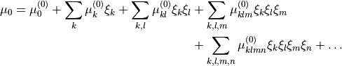
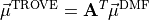
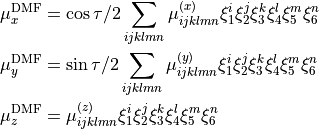
The functions $\mu_{\Gamma}^{\rm SMB}$ (henceforth referred to as $\mu_{\Gamma}$ ) are now represented as expansions:

$\begin{split} \mu_{A''_1} & = \cos\rho \left[ \mu_{0}^{(A''_1)} + \sum_{k} \mu_{k}^{(A''_1)} \xi_k + \sum_{k,l} \mu_{k,l}^{(A''_1)} \xi_k \xi_l + \sum_{k,l,m} \mu_{k,l,m}^{(A''_1)} \xi_k \xi_l \xi_m + \cdots \right] \\ \mu_{E'_a} & = \mu_{0}^{(E'_a)} + \sum_{k} \mu_{k}^{(E'_a)} \xi_k + \sum_{k,l} \mu_{k,l}^{(E'_a)} \xi_k \xi_l + \sum_{k,l,m} \mu_{k,l,m}^{(E'_a)} \xi_k \xi_l \xi_m + \cdots \\ \mu_{E'_b} = & \mu_{0}^{(E'_b)} + \sum_{k} \mu_{k}^{(E'_b)} \xi_k + \sum_{k,l} \mu_{k,l}^{(E'_b)} \xi_k \xi_l + \sum_{k,l,m} \mu_{k,l,m}^{(E'_b)} \xi_k \xi_l \xi_m + \cdots \end{split}$

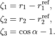
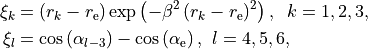
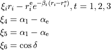
in terms of the variables

$\begin{split} \xi_k &= (r_k - r_{\rm e}) \exp \left[ -\beta \, (r_k-r_{\rm e})^2 \right], \;\; k=1,2,3, \\ \xi_{4}&= \frac{1}{\sqrt{6}} \left( 2 \alpha_{1} - \alpha_{2} - \alpha_{3} \right)\hbox{,} \\ \xi_{5}&= \frac{1}{\sqrt{2}} \left( \alpha_{2} - \alpha_{3} \right)\hbox{,} \\ \xi_{6} &= \sin\rho_{\rm e}-\sin\rho \hbox{,} \end{split}$

Here

$\sin {\rho} \, = \, \frac{2}{\sqrt{3}} \, \sin [ (\alpha_1 + \alpha_2 + \alpha_3) /6],$

and $\sin(\rho_{\rm e})$ is the equilibrium value of $\sin(\rho)$ . The factor 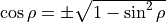$\cos\rho = \pm \sqrt{1-\sin^2 {\rho}}$ ensures that the dipole moment function $\mu_{A''_1}$ changes sign when $\rho = 0\ldots \pi$ is changed to $\pi - \rho$ . As in the rigid MB case, the factor $\exp \left[ -\beta (r_k-r_{\rm e})^2 \right]$ is used in order to keep the expansion from diverging at large $r_i$ .

Chain type ABCD-type molecules

`HOOH_MB`

Subroutine: MLdms_hooh_MB.

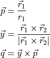
The DMF frame $xyz$ is defined with the $x$ axis as a bisector between two planes, H₁O₁O₂ and O₁O₂H₁ and $z$ axis along the O₁O₂ bond. Thus, the unit vector $k$ is defined as a normalised vector $\vec{r}_{12}$ , the unit vector $i$ is defined as a bisector between the normal to the planes 3-1-2 and 1-2-3 and the unit vector is defined via the rand-hand rule:

$\begin{split} \vec{k} &= \frac{\vec{r}_{12}}{r_{12}} \\ \vec{i} &= \frac{\vec{n}_1+\vec{n}_2}{|\vec{n}_1+\vec{n}_2|} \\ \vec{j} &= \vec{j}\times \vec{i} \end{split}$

where the plane normals are defined as follows:

$\begin{split} \vec{n}_1 &= \frac{\vec{r}_{21}\times \vec{r}_{12}}{|\vec{r}_{21}\times \vec{r}_{12}|} \\ \vec{n}_2 &= \frac{\vec{r}_{12}\times \vec{r}_{32}}{|\vec{r}_{12}\times \vec{r}_{32}|} \end{split}$

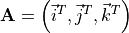
Here, the coordinate vectors $\vec{r}_{21}$ , $\vec{r}_{31}$ and $\vec{r}_{42}$ as well as $\vec{i}$ , $\vec{j}$ and $\vec{k}$ are given in the representation of the instantaneous TROVE frame $xyz$ . With this definition, the matrix constructed from these unit vecrtors $\vec{i}$ , $\vec{j}$ and $\vec{k}$ forms the rotation (unitary transformation) of the dipole vector between its original DMF frame and the instantaneous TROVE frame $xyz$ :

${\mathbf A} = \left( \vec{i}^T,\vec{j}^T,\vec{k}^T \right)$

and

$\vec{\mu}^{\rm TROVE} = {\mathbf A}^T \vec{\mu}^{\rm DMF}$

The $\mu_\alpha^{\rm DMF}$ are expressed as Taylor-type expansion:

$\begin{split} \mu_x^{\rm DMF} &= \cos\tau/2 \sum_{ijklmn} \mu_{ijklmn}^{(x)} \xi_1^i \xi_2^j \xi_3^k \xi_4^l \xi_5^m \xi_6^n \\ \mu_y^{\rm DMF} &= \sin\tau/2 \sum_{ijklmn} \mu_{ijklmn}^{(y)} \xi_1^i \xi_2^j \xi_3^k \xi_4^l \xi_5^m \xi_6^n \\ \mu_z^{\rm DMF} &= \mu_{ijklmn}^{(z)} \xi_1^i \xi_2^j \xi_3^k \xi_4^l \xi_5^m \xi_6^n \end{split}$

where

$\begin{split} \xi_i & r_i - r_{i}^{\rm e} e^{-\beta_i (r_i - r_{i}^{\rm e}) }, t=1,2,3 \\ \xi_4 & = \alpha_1 - \alpha_{\rm e} \\ \xi_5 & = \alpha_1 - \alpha_{\rm e} \\ \xi_6 & = \cos\delta \end{split}$

The expansion paramters are the subjetc to the permutation constraint:

$\begin{split} \mu_{i(jk)(lm)n}^{(x)} = \mu_{i(kj)(mn)n}^{(x)}, \quad {\rm for} j\ne k \quad l\ne m \\ \mu_{i(jk)(lm)n}^{(y)} = -\mu_{i(kj)(mn)n}^{(y)}, \quad {\rm for} j\ne k \quad l\ne m \\ \mu_{i(jk)(lm)n}^{(z)} = -\mu_{i(kj)(mn)n}^{(z)}, \quad {\rm for} j\ne k \quad l\ne m \end{split}$

This DMF form was used to produce the APTY line list for HOOH [15AlOvYu]. The TROVE input file describing this spectroscopic model can be found in APTY spectroscopic model. For this mode, the Dipole block is given by

Dipole
dimension 3
NPARAM     136   96   98
DMS_TYPE  HOOH_MB
COEFF   powers
COORDS  linear
Order   6 6 6
parameters
re1           0    0    0    0    0    0   0          1.45538654
re2           0    0    0    0    0    0   0          0.96257063
alphae        0    0    0    0    0    0   0        101.08307909
beta1         0    0    0    0    0    0   0          1.00000000
beta2         0    0    0    0    0    0   0          1.00000000
xxxxx         0    0    0    0    0    0   0          0.00000000
mu000000      0    0    0    0    0    0   7          3.11323258
mu000001      0    0    0    0    0    1   6         -0.05725254
mu000002      0    0    0    0    0    2   5         -0.00374176
mu000003      0    0    0    0    0    3   4         -0.0048
....

where dimension is 3.

`HPPH_MB`

Subroutine: MLdms_hpph_MB

See ./input/39K-16O-1H__OYT4_model_TROVE.inp

HCCH_MB
HCCH_DMS_7D
HCCH_DMS_7D_7ORDER
HCCH_DMS_7D_7ORDER_LINEAR
HCCH_DMS_7D_LOCAL
HCCH_ALPHA_ISO_7D_LINEAR

ZXY₂

ZXY2_SYMADAP

ZXY₃

ZXY3_SYM

C₂H₄

DIPOLE_C2H4_4M

Properties

XY2_SR-BISECT
XY2_SS_DIPOLE_YY

XY2_G-BISECT
XY2_G-ROT-ELEC
XY2_G-COR-ELEC
XY2_G-TENS-RANK3
XY2_G-TENS-NUC
XY3_NSS_MB
COORDINATES

Dipole moment functions

Dipole (External) Block

Implemented DMFs

XY2 type

xy2_pq_coeff

XY2_PQ_LINEAR

DIPOLE_AMES1

DIPOLE_SO2_AMES1

XY2_C3_SCHROEDER

DIPOLE_PQR_XYZ_Z-FRAME

DIPOLE_PQR_XYZ_Z-FRAME_SINRHO