Rigid triatomic molecule XY₂

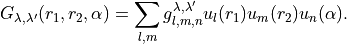
Consider a triatomic molecule in a rigid representation and a bisector frame. Ignoring singularity at the linearity, we derive an analytic expression for the KEO in the valence coordinates $r_1$ , $r_2$ , $\alpha$ and represent it as the following basic-functions expansions:

(1) $G_{\lambda,\lambda'}(r_1,r_2,\alpha) = \sum_{l,m} g_{l,m,n}^{\lambda,\lambda'} u_{l}(r_1) u_{m}(r_2) u_{n}(\alpha).$

For the basis functions, only the following basic functions are needed:

for bond-lengths $r_1$ and $r_2$

Index	Term
1	$1/r$
2	$1/r^2$

for the bond angle

Basic-functions block

for this types of the expansion basic-function terms, the Basic-function structure is given by

Two stretching modes:

		mode	$N_{\rm func}$
	`Mode`	1,2	2
#	$N_{\rm contr}$	$n_i$	type	$a_i$	$k_i$
1	1 and 2	-1	I	1	1
2	1 and 2	-2	I	1	1

Bending mode:

		mode	$N_{\rm func}$
	`Mode`	3	6
#	$N_{\rm contr}$	$n_i$	type	$a_i$	$k_i$
1	1	2	Cos	0.5	1
2	1	2	sec	0.5	1
3	1	2	Csc	0.5	1
4	1	1	Sin	1	1
5	1	2	sec	1	1
6	2	2	Cot	0.5	1

The Basic-function block is then given by

BASIC-FUNCTION
Mode 1 2
1 1 -1 I 1 1
2 1 -2 I 1 1
Mode 2 2
1 1 -1 I 1 1
2 1 -2 I 1 1
Mode 3 6
1 1 2 Cos 0.5 1
2 1 2 Sec 0.5 1
3 1 2 Csc 0.5 1
4 1 1 sin 1.0 1
5 1 1 sec 1.0 1
6 1 2 cot 0.5 1
END

The corresponding “kinetic” card in the Basis block must be set to automatic:

BASIS
 0,'JKtau', Jrot 0
 1,'numerov','automatic', 'morse', range 0,  4,  resc 1.0, points 600,borders -0.5,1.40
 1,'numerov','automatic', 'morse', range 0,  4,  resc 1.0, points 600,borders -0.5,1.40
 2,'numerov','automatic', 'linear', range 0, 4,  resc 1.0, points 500,borders   -60.0,60.0 deg
END

Kinetic energy operator

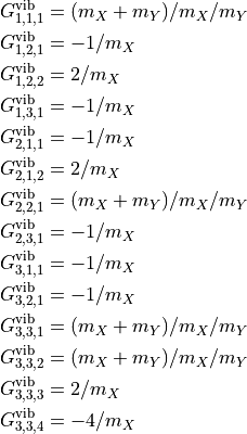
The corresponding KEO expansion terms are given by (before multiplying with $\hbar^2/2$ ):

Vibrational part:

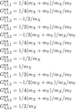
$\begin{split} G^{\rm vib}_{1,1,1} &= (m_X+m_Y)/m_X/m_Y \\ G^{\rm vib}_{1,2,1} &= -1/m_X \\ G^{\rm vib}_{1,2,2} &= 2/m_X \\ G^{\rm vib}_{1,3,1} &= -1/m_X \\ G^{\rm vib}_{2,1,1} &= -1/m_X \\ G^{\rm vib}_{2,1,2} & = 2/m_X \\ G^{\rm vib}_{2,2,1} & = (m_X+m_Y)/m_X/m_Y\\ G^{\rm vib}_{2,3,1} & = -1/m_X \\ G^{\rm vib}_{3,1,1} & = -1/m_X \\ G^{\rm vib}_{3,2,1} & = -1/m_X \\ G^{\rm vib}_{3,3,1} & = (m_X+m_Y)/m_X/m_Y\\ G^{\rm vib}_{3,3,2} & = (m_X+m_Y)/m_X/m_Y\\ G^{\rm vib}_{3,3,3} & = 2/m_X \\ G^{\rm vib}_{3,3,4} & = -4/m_X \\ \end{split}$

Rotational part:

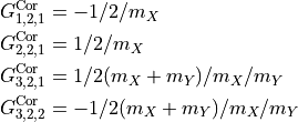
$\begin{split} G^{\rm rot}_{1,1,1} & = 1/4(m_X+m_Y)/m_X/m_Y \\ G^{\rm rot}_{1,1,2} & = 1/4(m_X+m_Y)/m_X/m_Y \\ G^{\rm rot}_{1,1,3} & = -1/2/m_X \\ G^{\rm rot}_{1,3,1} & = 1/2(m_X+m_Y)/m_X/m_Y \\ G^{\rm rot}_{1,3,2} & = -1/2(m_X+m_Y)/m_X/m_Y \\ G^{\rm rot}_{2,2,1} & = 1/4(m_X+m_Y)/m_X/m_Y \\ G^{\rm rot}_{2,2,2} & = 1/4(m_X+m_Y)/m_X/m_Y \\ G^{\rm rot}_{2,2,3} & = -1/2/m_X \\ G^{\rm rot}_{2,2,4} & = 1/m_X \\ G^{\rm rot}_{3,1,1} & = 1/2(m_X+m_Y)/m_X/m_Y \\ G^{\rm rot}_{3,1,2} & = -1/2(m_X+m_Y)/m_X/m_Y \\ G^{\rm rot}_{3,3,1} & = 1/4(m_X+m_Y)/m_X/m_Y \\ G^{\rm rot}_{3,3,2} & = 1/4(m_X+m_Y)/m_X/m_Y \\ G^{\rm rot}_{3,3,3} & = 1/2/m_X \\ \end{split}$

Coriolis part:

$\begin{split} G^{\rm Cor}_{1,2,1} & = -1/2/m_X \\ G^{\rm Cor}_{2,2,1} & = 1/2/m_X \\ G^{\rm Cor}_{3,2,1} & = 1/2(m_X+m_Y)/m_X/m_Y \\ G^{\rm Cor}_{3,2,2} & = -1/2(m_X+m_Y)/m_X/m_Y \\ \end{split} \\$

Pseudo potential:

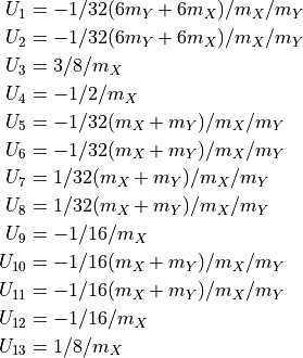
$\begin{split} U_{1} & = -1/32(6m_Y+6m_X)/m_X/m_Y \\ U_{2} & = -1/32(6m_Y+6m_X)/m_X/m_Y \\ U_{3} & = 3/8/m_X \\ U_{4} & = -1/2/m_X \\ U_{5} & = -1/32(m_X+m_Y)/m_X/m_Y \\ U_{6} & = -1/32(m_X+m_Y)/m_X/m_Y \\ U_{7} & = 1/32(m_X+m_Y)/m_X/m_Y \\ U_{8} & = 1/32(m_X+m_Y)/m_X/m_Y \\ U_{9} & = -1/16/m_X \\ U_{10} & = -1/16(m_X+m_Y)/m_X/m_Y \\ U_{11} & = -1/16(m_X+m_Y)/m_X/m_Y \\ U_{12} & = -1/16/m_X \\ U_{13} & = 1/8/m_X \\ \end{split}$

The highest expansion term is 13 (pseudo-potential function). This value must be used for the NKinOrder card:

KinOrder   13

There are methods this KEO can be used in TROVE.

Using kinetic.chk. To this end, the expansion terms must be numerically evaluated for the given set of the nuclear mass and listed kinetic.chk using the format explained in Kinetic energy operators.

2. It can be also implemented directly into the kin_xy2.f90 module. For this example, the KEO has been implemented as KINETIC_XY2_EKE_BISECT_COMPACT_RIGID and can be used as follows:

KINETIC
  compact
  kinetic_type  KINETIC_XY2_EKE_BISECT_COMPACT_RIGID
END

Here the card compact is to indicate the special “compact” format associated with the basic-function expansion. If this compact form of the analytic KEO is used, the kinetic.chk checkpoint file will be created using the basic-function format with all the modes specified explicitly, so that it can read using method 1.

Input Example for H₂S

An example of this KEO for H₂S can be found in H2S_EKE_basic-functions_step1.inp. It has the following format.

Basic control parameter:

KinOrder   13
PotOrder   8

Natoms 3
Nmodes 3

sparse

Size of the primitive and contracted basis sets:

PRIMITIVES
  Npolyads  4
END

CONTRACTION
  Npolyads      4
  sample_points   40
END

Symmetry

SYMGROUP C2v(M)

Frame and definition of the coordinates:

COORDS CURVILINEAR
TRANSFORM  r-alpha
frame  bisect-z
MOLTYPE XY2
REFER-CONF RIGID

Z-matrix and atomic masses

ZMAT
    S   0  0  0  0  31.97207070
    H   1  0  0  0   1.00782505
    H   1  2  0  0   1.00782505
end

Definition of the individual 1D basis set and expansion functions, including automatic as associated with the basis-function option.

BASIS
 0,'JKtau', Jrot 0
 1,'numerov','automatic', 'morse', range 0,  4,  resc 1.0, points 600,borders -0.5,1.40
 1,'numerov','automatic', 'morse', range 0,  4,  resc 1.0, points 600,borders -0.5,1.40
 2,'numerov','automatic', 'linear', range 0, 4,  resc 1.0, points 500,borders   -60.0,60.0 deg
END

Basic-function block:

BASIC-FUNCTION
Mode 1 2
1 1 -1 I 1 1
2 1 -2 I 1 1
Mode 2 2
1 1 -1 I 1 1
2 1 -2 I 1 1
Mode 3 6
1 1 2 Cos 0.5 1
2 1 2 Sec 0.5 1
3 1 2 Csc 0.5 1
4 1 1 sin 1.0 1
5 1 1 sec 1.0 1
6 1 2 cot 0.5 1
END

Kinetic energy operator block:

KINETIC
  compact
  kinetic_type  KINETIC_XY2_EKE_BISECT_COMPACT_RIGID
END

Control block:

control
step 1
end

Equilibrium and special parameters blocks:

EQUILIBRIUM
re13       1         1.3359007d0
re13       1         1.3359007d0
alphae     0         92.265883d0  DEG
end

SPECPARAM
aa         0         1.70400000d0
aa         0         1.70400000d0
END

Potential energy function block:

POTEN
POT_TYPE  poten_xy2_tyuterev
COEFF  list  (powers or list)
b1        0    0.80000000000000E+06
b2        0    0.80000000000000E+05
g1        0    0.13000000000000E+02
g2        0    0.55000000000000E+01
f000      0    0.00000000000000E+00
f001      1    0.25298724728304E+01
f100      1    0.76001446034650E+01
......
end

DMF block

DIPOLE   (CCSD(T)/aug-cc-pV(6+d)Z)
  rank 3
  NPARAM  72 99 0
  TYPE  xy2_pq_coeff
  COEFF   list  (powers or list)
  COORDS  linear linear linear
  Orders  10 10  10
  Parameters
  re            0      0.133600000000E+01
  alphae        0      0.922000000000E+02
  f03y1y0y0     7       0.00478832298768
  f04y1y0y1     7      -0.76979371155700
  f05y2y0y0     6      -0.23510259705300
  f06y1y0y2     6       0.22148707034900
  f07y2y0y1     6       0.39210356641800
  ......
  end

Rigid triatomic molecule XY2

Basic-functions block

Kinetic energy operator

Input Example for H2S

Rigid triatomic molecule XY₂

Input Example for H₂S